Seldonian ML
GitHub
Tutorial E: Predicting student GPAs from application materials with fairness guarantees
Contents
Introduction
One of the examples presented by Thomas et al. (2019) explores enforcing five popular definitions of fairness on a classification problem. The classification problem involves predicting whether students have higher ($\geq3.0$) or lower ($<3.0$) grade point averages (GPAs) based on their scores on nine entrance examinations. Thomas et al. used custom code that predates the Seldonian Toolkit to run their Seldonian algorithms. In this tutorial, we will demonstrate how to use the Seldonian Toolkit to apply the same fairness definitions to the same dataset. Specifically, we will run Seldonian Experiments, recreating the plots in Figure 3 of their paper.
Caveats
- The Seldonian Toolkit currently only supports quasi-Seldonian algorithms, so we will not recreate the curves labeled "Seldonian classification" by Thomas et al. (2019) in their Figure 3.
- Version 0.2.0 of Fairlearn, the version used by Thomas et al. and the first publicly released version, is not compatible with Python 3.8, the minimum version of Python supported by the Seldonian Toolkit. Instead, we used the most recent stable version of Fairlearn (0.7.0) to run the code in this tutorial. The Fairlearn API has evolved considerably since 0.2.0, and it now supports more of the fairness constraints considered by Thomas et al. (2019).
- In candidate selection, we used gradient descent with a logistic regression model, whereas Thomas et al. (2019) used black box optimization with a linear classifier model to find the candidate solution. This may change how much data it takes for the performance and solution rate of the quasi-Seldonian models to achieve the optimal values, but the overall trends should not be affected.
- We used 50 trials per data fraction in our experiments, compared to Thomas et al. (2019) who used 250 trials per data fraction. This only has the effect of increasing our uncertainty ranges compared to theirs. The overall trends are not affected.
For all of these reasons, we seek to reproduce the general trends found by Thomas et al. (2019) rather than the identical results.
Outline
In this tutorial, you will learn how to:
- Format the GPA classification dataset used by Thomas et al. (2019) for use in the Seldonian Toolkit.
- Create the three plots of a Seldonian Experiment for the five different fairness definitions considered by Thomas et al. (2019).
Dataset preparation
We created a Jupyter notebook implementing the steps described in this section. If you would like to skip this section, you can find the correctly reformatted dataset and metadata files that are the end product of the notebook here: https://github.com/seldonian-toolkit/Engine/tree/main/static/datasets/supervised/GPA.
We downloaded the GPA dataset file called data.csv from the Harvard dataverse link listed by Thomas et al. (2019). Specifically, we followed that link and then clicked the "Access Dataset" dropdown and downloaded the "Original Format ZIP (3.0 MB)" file. At that link, there is a description of the columns. We used the pandas library to load the CSV file into a dataframe. We scaled the columns representing the nine entrance exam scores using a standard scaler. We then created a new column called GPA_class to which we assigned a value of 1 if the existing GPA column had a value $\geq3$ and assigned a value of 0 otherwise. While the dataset already has a gender column, the Seldonian Toolkit requires each group in a sensitive attribute to have its own binary-valued column. As a result, we created two new columns, "M" (male) and "F" (female) from the values of the gender column. We set the values of the "M" column to be 1 if the gender was male and 0 if female. For the "F" column, we set the values to be 1 if the gender was female and 0 if male. Finally, we dropped the original gender and GPA columns, reordered the columns so that the sensitive attributes were first, followed by the scaled test scores, followed by the GPA_class label column, and saved the file in CSV format. This file can be found here. We also created a JSON file containing the metadata that we will provide to the Seldonian Engine library here.
Thomas et al. (2019) considered five different definitions of fairness to apply to the problem of predicting whether students would have high or low GPAs based on nine entrance examination scores. The five definitions, and their constraint strings are:
- Disparate impact: 'min((PR | [M])/(PR | [F]),(PR | [F])/(PR | [M])) >= 0.8'
- Demographic parity: 'abs((PR | [M]) - (PR | [F])) <= 0.2'
- Equalized odds: 'abs((FNR | [M]) - (FNR | [F])) + abs((FPR | [M]) - (FPR | [F])) <= 0.35'
- Equal opportunity: 'abs((FNR | [M]) - (FNR | [F])) <= 0.2'
- Predictive equality: 'abs((FPR | [M]) - (FPR | [F])) <= 0.2'
They applied each of these constraints independently, each with $\delta=0.05$.
Creating the specification object
We need to create a different spec object for each constraint because we will be running five different experiments. However, every other input to the spec object is the same, so we can make five spec objects using a for loop. In the script below, set data_pth and metadata_pth to point to where you saved the data and metadata files from above. save_base_dir is the parent directory to where five directories will be created, one holding each spec object. Change it to somewhere convenient on your machine.
Note: Comparing this script to the equivalent one in the fair loans tutorial, you may notice that the model and primary objective are missing here. That is because we are using a wrapper function called createSupervisedSpec() here which fills in the default values for these quantities in the classification setting, i.e., a logistic regression model with log loss.
# createSpec.py
import os
from seldonian.parse_tree.parse_tree import make_parse_trees_from_constraints
from seldonian.dataset import DataSetLoader
from seldonian.utils.io_utils import (load_json,save_pickle)
from seldonian.spec import createSupervisedSpec
from seldonian.models.models import (
    BinaryLogisticRegressionModel as LogisticRegressionModel)
from seldonian.models import objectives

if __name__ == '__main__':
    data_pth = "../../static/datasets/supervised/GPA/gpa_classification_dataset.csv"
    metadata_pth = "../../static/datasets/supervised/GPA/metadata_classification.json"
    save_base_dir = '../../../interface_outputs'
    # save_base_dir='.'
    # Load metadata
    regime='supervised_learning'
    sub_regime='classification'

    loader = DataSetLoader(
        regime=regime)

    dataset = loader.load_supervised_dataset(
        filename=data_pth,
        metadata_filename=metadata_pth,
        file_type='csv')

    # Behavioral constraints
    deltas = [0.05]
    for constraint_name in ["disparate_impact",
        "demographic_parity","equalized_odds",
        "equal_opportunity","predictive_equality"]:
        save_dir = os.path.join(save_base_dir,f'gpa_{constraint_name}')
        os.makedirs(save_dir,exist_ok=True)
        # Define behavioral constraints
        if constraint_name == 'disparate_impact':
            constraint_strs = ['min((PR | [M])/(PR | [F]),(PR | [F])/(PR | [M])) >= 0.8']
        elif constraint_name == 'demographic_parity':
            constraint_strs = ['abs((PR | [M]) - (PR | [F])) <= 0.2']
        elif constraint_name == 'equalized_odds':
            constraint_strs = ['abs((FNR | [M]) - (FNR | [F])) + abs((FPR | [M]) - (FPR | [F])) <= 0.35']
        elif constraint_name == 'equal_opportunity':
            constraint_strs = ['abs((FNR | [M]) - (FNR | [F])) <= 0.2']
        elif constraint_name == 'predictive_equality':
            constraint_strs = ['abs((FPR | [M]) - (FPR | [F])) <= 0.2']

        createSupervisedSpec(
            dataset=dataset,
            metadata_pth=metadata_pth,
            constraint_strs=constraint_strs,
            deltas=deltas,
            save_dir=save_dir,
            save=True,
            verbose=True)
Running this code should print out that the five spec files have been created.
Running a Seldonian Experiment
To produce the three plots, we will run a Seldonian Experiment using a quasi-Seldonian model, a baseline logistic regression model, and a Fairlearn model with three different values of epsilon (0.01,0.1,1.0) in the constraint in order to match Thomas et al. (2019). We used the same performance metric as Thomas et al. (2019), deterministic accuracy, i.e, $1-\frac{1}{m}\sum_{i=1}^{m}(\hat{y}_i(\theta,X_i) \neq Y_i)$, where $m$ is the number of data points in the entire dataset, $Y_i$ is the label for the $i$th data point and $\hat{y}_i(\theta,X_i)$ is the model prediction for the $i$th data point, given the data point $X_i$ and the model parameters $\theta$. Here is the code we used to produce the plot for disparate impact:
# generate_gpa_plots.py
import os
# this line disables NumPy's implicit parallelization
# and speeds up our own parallelization of experiments
os.environ["OMP_NUM_THREADS"] = "1"
import numpy as np

from experiments.generate_plots import SupervisedPlotGenerator
from seldonian.utils.io_utils import load_pickle
from sklearn.metrics import log_loss,accuracy_score

from experiments.baselines.logistic_regression import BinaryLogisticRegressionBaseline

if __name__ == "__main__":
    # Parameter setup
    run_experiments = True
    make_plots = True
    save_plot = True
    include_legend = True
    constraint_name = 'disparate_impact'
    fairlearn_constraint_name = constraint_name
    fairlearn_epsilon_eval = 0.8 # the epsilon used to evaluate g, needs to be same as epsilon in our definition
    fairlearn_eval_method = 'two-groups' # the epsilon used to evaluate g, needs to be same as epsilon in our definition
    fairlearn_epsilons_constraint = [0.01,0.1,1.0] # the epsilons used in the fitting constraint
    performance_metric = 'accuracy'
    n_trials = 50
    data_fracs = np.logspace(-4,0,15)
    n_workers = 8
    results_dir = f'results/gpa_{constraint_name}_{performance_metric}_2022Nov15'
    plot_savename = os.path.join(results_dir,f'gpa_{constraint_name}_{performance_metric}.png')

    verbose=True

    # Load spec
    specfile = f'../interface_outputs/gpa_{constraint_name}/spec.pkl'
    spec = load_pickle(specfile)

    os.makedirs(results_dir,exist_ok=True)

    # Use entire original dataset as ground truth for test set
    dataset = spec.dataset
    test_features = dataset.features
    test_labels = dataset.labels

    # Setup performance evaluation function and kwargs
    # of the performance evaluation function

    def perf_eval_fn(y_pred,y,**kwargs):
        if performance_metric == 'log_loss':
            return log_loss(y,y_pred)
        elif performance_metric == 'accuracy':
            return accuracy_score(y,y_pred > 0.5)

    perf_eval_kwargs = {
        'X':test_features,
        'y':test_labels,
        }

    plot_generator = SupervisedPlotGenerator(
        spec=spec,
        n_trials=n_trials,
        data_fracs=data_fracs,
        n_workers=n_workers,
        datagen_method='resample',
        perf_eval_fn=perf_eval_fn,
        constraint_eval_fns=[],
        results_dir=results_dir,
        perf_eval_kwargs=perf_eval_kwargs,
        )

    # # Baseline models
    if run_experiments:

        plot_generator.run_baseline_experiment(
            baseline_model=BinaryLogisticRegressionBaseline(),verbose=True)

        # Seldonian experiment
        plot_generator.run_seldonian_experiment(verbose=verbose)


    ######################
    # Fairlearn experiment
    ######################

    fairlearn_sensitive_feature_names=['M']

    # Make dict of test set features, labels and sensitive feature vectors

    fairlearn_sensitive_feature_names = ['M']
    fairlearn_sensitive_col_indices = [dataset.sensitive_col_names.index(
        col) for col in fairlearn_sensitive_feature_names]
    fairlearn_sensitive_features = dataset.sensitive_attrs[:,fairlearn_sensitive_col_indices]
    # Setup ground truth test dataset for Fairlearn
    test_features_fairlearn = test_features
    fairlearn_eval_kwargs = {
        'X':test_features_fairlearn,
        'y':test_labels,
        'sensitive_features':fairlearn_sensitive_features,
        'eval_method':fairlearn_eval_method,
        'performance_metric':performance_metric,
        }

    if run_experiments:
        for fairlearn_epsilon_constraint in fairlearn_epsilons_constraint:
            plot_generator.run_fairlearn_experiment(
                verbose=verbose,
                fairlearn_sensitive_feature_names=fairlearn_sensitive_feature_names,
                fairlearn_constraint_name=fairlearn_constraint_name,
                fairlearn_epsilon_constraint=fairlearn_epsilon_constraint,
                fairlearn_epsilon_eval=fairlearn_epsilon_eval,
                fairlearn_eval_kwargs=fairlearn_eval_kwargs,
                )

    if make_plots:
        plot_generator.make_plots(fontsize=12,legend_fontsize=12,
            performance_label=performance_metric,
            performance_yscale='log',
            savename=plot_savename if save_plot else None,
            save_format="png")
Save the code above as a file called: generate_gpa_plots.py and run the script from the command line like:
$ python generate_gpa_plots.py
To run the experiment for the other constraints, at the top of the file change constraint_name to the other constraint names: demographic_parity, equalized_odds, equal_opportunity, and predictive_equality. For each constraint, make sure fairlearn_constraint_eval is set correctly. This value needs to be the threshold value in the corresponding constraint string. It is 0.35 for equalized odds and 0.2 for the three other remaining constraints. Rerun the script for each constraint.
Running the script for each constraint will produce the following plots:
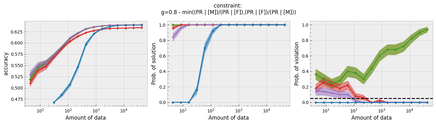
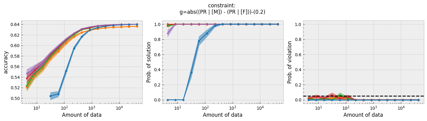
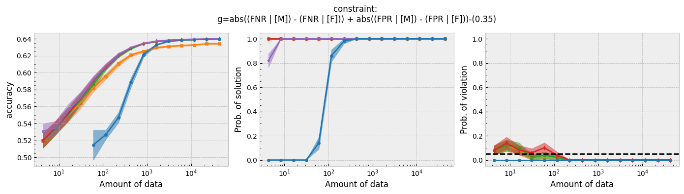
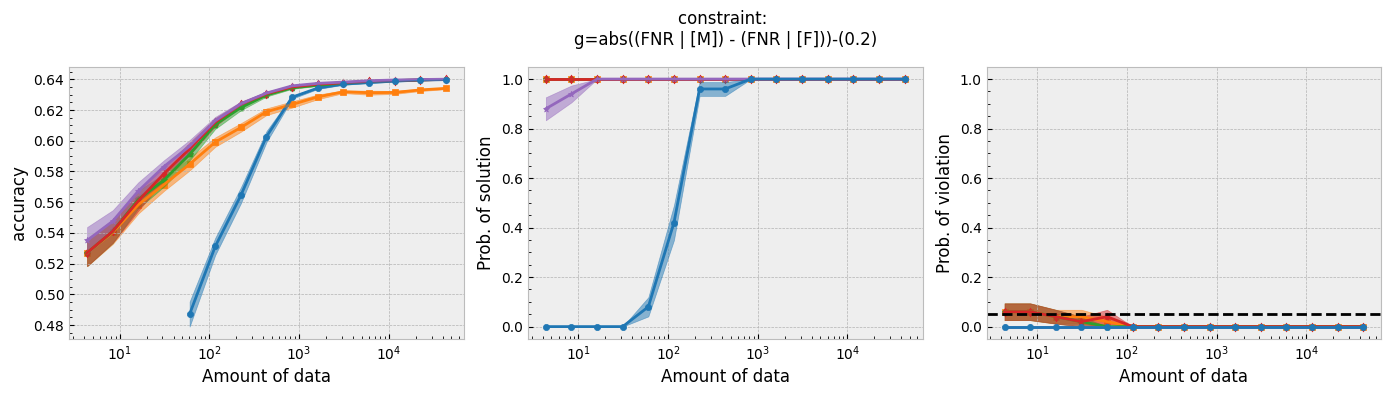
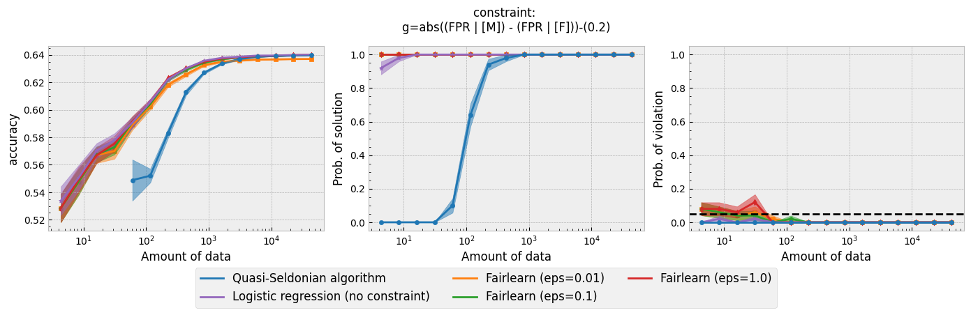 Figure 1 - The three plots of a Seldonian Experiment, accuracy (left), solution rate (middle) and failure rate (right), for five different fairness constraints enforced independently on the GPA classification dataset considered by Thomas et al. (2019). The colored points and bands in each panel show the mean standard error over 50 trials. Each row of plots is an experiment for a different fairness constraint. From top to bottom: disparate impact, demographic parity, equalized odds, equal opportunity, predictive equality. The legend in the bottom panel applies to all five panels. A quasi-Seldonian algorithm (qsa, blue) is compared to a logistic regression baseline (magenta), as well as a Fairlearn model enforcing the constraints above with three different values of the group disparity threshold, $\epsilon$: 0.01 (orange), 0.1 (green), and 1.0 (red). Note that the vertical axis range is [0,1] for failure rate on all subplots, whereas Thomas et al. (2019), Figure 3 shows a smaller range that varies for the different constraints.
While the QSA requires the most samples to return a solution and to achieve optimal accuracy, it is the only model that always satisfies the fairness constraints regardless of the number of samples. We observe the same general trends for the QSA here that Thomas et al. (2019) saw for all five fairness constraints. Our QSA models require slightly fewer data points than theirs to achieve optimal performance and a solution rate of 1.0. This is likely due to the difference in the optimization strategies for candidate selection. We used KKT optimization (modified gradient descent), whereas Thomas et al. (2019) used black box optimization. Both methods are equally valid. In fact, any algorithm is valid for candidate selection (that is, it will not cause the algorithm to violate its safety guarantee) as long as it does not use any of the safety data.
The largest differences between our experiments and those done by Thomas et al. are in the Fairlearn results. The newer Fairlearn models that we ran achieve near-optimal accuracy with almost any amount of data. The older Fairlearn models never reached optimal accuracy in the experiments performed by Thomas et al. The Fairlearn API has changed considerably since Thomas et al. used it, and more fairness constraints can be included in their models. That being said, their models continue to violate the fairness constraints. In particular, the disparate impact constraint is violated with high probability over the most of the sample sizes considered. This is not surprising given that the Fairlearn models do not have a safety test; their models make no guarantee that they will not violate the constraints on unseen data.
Summary
In this tutorial, we demonstrated how to use the Seldonian Toolkit to recreate the analysis performed by Thomas et al. (2019) using the GPA classification dataset. In particular, we sought to recreate their Figure 3. We showed how to format the dataset so that it can be used in the Seldonian Toolkit. Using the same five fairness constraints that Thomas et al. (2019) considered, we ran a Seldonian Experiment for each constraint. We produced the three plots: accuracy, solution rate, and failure rate, finding similar overall trends as Thomas et al. The quasi-Seldonian algorithms we ran slightly outperformed those run by Thomas et al. (2019), but in general were very similar. The main differences we found were in the Fairlearn models. The differences we observed are easily explained by updates to the Fairlearn API that took place since 2019. Due to compatibility issues, we were unable to use the same Fairlearn API version as Thomas et al. with the newer Python versions required by the Seldonian Toolkit.