Seldonian ML
GitHub
Tutorial L: Creating Fair Decision Trees and Random Forests (for binary classification)
Contents
Introduction
For tabular datasets, tree-based models are often the first choice for ML practitioners. Depending on the specific model, they can have advantages, such as explainability, a smaller memory footprint, and lower latency (both at training and inference time), compared to more complex models like artificial neural networks. There are many types of tree-based models, but at the foundation of all of them is the decision tree.
As with most standard ML models, simply training a decision tree using an off-the-shelf algorithm such as Classification And Regression Trees (CART; Breiman et al. 1984) can lead to a model that makes unfair predictions with respect to sensitive attributes (e.g., race, gender), even when those attributes are not explictly used as features in the dataset. In the context of the Seldonian Toolkit, this means that if we use CART during candidate selection, the safety test is unlikely to pass, though the likelihood of the safety test passing is of course dependent on the strictness of the behavioral constraints. We want candidate selection to be effective at enforcing any set of behavioral constraints, while simultaneously optimizing for the primary objective (e.g., accuracy). When it is not possible to satisfy the behavioral constraints, the safety test will inform us of this.
The methods we have found to be effective for general-purpose candidate selection assume parametric models (for details, see the algorithm details tutorial). Tree-training algorithms like CART are incompatible with these techniques because the trees they train are non-parameteric. Rather than alter CART, our approach is to take an already-built decision tree and run a second optimization procedure on it. In a typical decision tree, a label is assigned to each leaf node. During the second optimization procedure, we assign probabilities for every label to each leaf node and optimize these probabilities. Tuning the label probabilities for each leaf node can be viewed as training a parametric model (the parameters determine the probabilities of each label in each leaf node), and so the existing Seldonian algorithm machinery in the toolkit for training parametric models while taking into account behavioral constraints can be applied directly. The result is a general-purpose Seldonian decision tree (SDTree) model that can be used to ensure that behavioral constraints are satisfied with high-confidence on tabular problems. The approach can also be used for other tree-based models, and we will cover how to extend it to random forests in this tutorial.
There are many approaches proposed in the literature for creating fairness-aware decision trees, including similar leaf-tuning techniques (e.g., Kamiran et al., 2010 and Aghaei et al., 2019). However, as far as we are aware, none of the existing methods provide high-confidence guarantees of fairness. Similarly, none of the existing methods work for definitions of fairness that are dynamically defined, like what is possible with the Seldonian Toolkit.
Note 1: The models discussed in this tutorial are only designed for binary classification problems. With some modification, they could be used for regression and multi-class classification problems.
Note 2: While the approach in this tutorial is agnostic to the algorithm or library used to build the initial decision tree, in practice we use scikit-learn, which implements a variation on the CART algorithm to build its trees. In order to use other libraries for building the initial tree model, a small amount of plug-in code is required to make the model compatible the toolkit (see the section How does the SDTree model work? below for details). If this is something you would find valuable, please open an issue or submit a pull request.
Outline
In this tutorial, we will:
- Cover how the SDTree is trained in candidate selection.
- Explain how the SDTree can be extended to a Seldonian Random Forest (SRF).
- Apply the SDTree and SRF to the GPA prediction problem from Tutorial E.
How does the SDTree model work?
Note: this section is quite technical, and reading it in its entirety is not necessary for simply using the SDTree model. This section is intended for developers who are seeking to modify or better understand this model.
In brief, the Seldonian decision tree model relabels the leaf node label probabilities so that the model's predictions enforce the behavioral constraints while maintaining high accuracy.
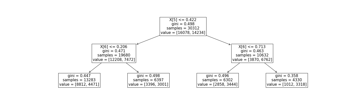 Figure 1 - A simple decision tree with
 max_depth=2 built using scikit-learn's DecisionTreeClassifier on a binary classification problem. Each internal node (including the root node) displays the feature split condition, the gini index, the number of samples that reach the node, and a "value" vector. Each leaf node displays the gini index, the number of samples that reach the node, and a "value" vector. For internal nodes, the first element of the value vector is the number of samples that meet the split condition, and the second number is the number that do not. For leaf nodes, the two numbers in the value vector indicate the number of samples whose true labels are 0 and 1, respectively.
Let's assume we have obtained the decision tree in Figure 1 by training an instance of scikit-learn's DecisionTreeClassifier on some imaginary tabular dataset. Our goal is to enforce behavioral constraints on this model with high confidence. First, we obtain the probabilities of predicting the positive and negative class in each leaf node. The most straightforward way to do this is to consider the probabilities to be the fraction of samples that reach the leaf node that belong to each true label class (in this case, 0 or 1). Taking the left-most leaf node as an example, the probabilities for predicting the 0th and 1st classes are:
$$ \Pr(\hat{y} = 0) = \frac{8812}{8812+4471} \approx 0.66 $$
$$ \Pr(\hat{y} = 1) = \frac{4471}{8812+4471} \approx 0.34 $$
Because these probabilities are redundant (i.e., $ \Pr(\hat{y} = 1) = 1.0 - \Pr(\hat{y} = 0)$), we only need to compute one of them for each leaf node. Our convention is to only compute $\Pr(\hat{y} = 1)$. The probabilities of each leaf node are what we want to tune using the KKT optimization procedure subject to our behavioral constraint(s). However, probabilities are bounded between 0 and 1, and the optimization procedure works best with unbounded parameters. Therefore, for the $j$th leaf node, we define a parameter, $\theta_j \in (-\infty,\infty)$, such that:
$$
\begin{equation}
\Pr(\hat{y} = 1)_j = \sigma\left(\theta_j\right) = \frac{1}{1+e^{-\theta_j}},
\label{theta2probs}
\end{equation}
$$
which ensures that $\Pr(\hat{y} = 1)_j \in (0,1)$. We can also express $\theta_j$ in terms of $\Pr(\hat{y} = 1)_j$:
$$
\begin{equation} \theta_j = \ln\left(\frac{1}{\frac{1}{\Pr(\hat{y} = 1)_j}-1}\right) \label{probs2theta}
\end{equation}
$$
As a result, the length of our parameter vector $\theta$ is the number of leaf nodes in the tree. We initialize $\theta$ using the probabilites of the decision tree that was fit by scikit-learn, mapping from probabilities to $\theta$ using Equation \ref{probs2theta}. At each step in the KKT optimization, we take the updated value of $\theta$, map it back to $\Pr(\hat{y} = 1)$ for each leaf node using Equation \ref{theta2probs}, and update the leaf node probabilities in the tree. We then make predictions using the updated tree. We repeat this process until the stopping criteria of the KKT procedure are met.
The KKT optimization procedure uses the gradients of the primary objective and the upper bound on the constraint functions to take steps in parameter space. Both of the functions whose gradients are needed involve a forward pass of the decision tree. In the toolkit, these gradients are calculated using the autograd library, which (with some exceptions for NumPy and SciPy) is incompatible with external libraries such as scikit-learn. A way around this is to manually define the gradient of the forward pass, or more specifically the Jacobian matrix, and then instruct autograd to use the manual definition of the gradient. Fortunately, the Jacobian is straightforward in this case. Consider what the forward pass $d(X_i,\theta)$ of this model does: for a given input data sample $X_i$, it computes the probability of classifying that sample into the positive class, i.e. $d(X_i,\theta) = \Pr(\hat{y}(X_i,\theta) = 1)$. The elements of the Jacobian matrix can then be written:
$$
\begin{equation}
J_{i,j}=\frac{\partial \left( \Pr(\hat{y}(X_i,\theta) = 1) \right)}{\partial \theta_j}
\end{equation}
\label{Jacobian}
$$
If there are M data samples and N leaf nodes, the Jacobian is a MxN matrix. Because the $\theta$ vector consists of a list of the leaf node probabilities (after transformation via Equation \ref{probs2theta}), an element $J_{i,j}$ of the Jacobian has a value of 1 when the leaf node that is hit by sample $i$ has the probability value mapped from the corresponding value $\theta_j$ via Equation \ref{theta2probs}, and 0 otherwise. Therefore, each row of the Jacobian is a one-hot vector (i.e., has a single value of 1 and is 0 otherwise).
To make this more concrete, consider the decision tree in Figure 1 and the first 3 samples of an imaginary dataset. If the first sample's decision path through the tree ends at the second leaf node (from the left), the second sample ends at the first leaf node, and the third sample ends at the final (fourth) leaf node, the first 3 rows of the Jacobian would look like this:
[
    [0, 1, 0, 0],
    [1, 0, 0, 0],
    [0, 0, 0, 1],
    ...
]
We implemented a Seldonian decision tree model that uses scikit-learn's DecisionTreeClassifier as the initial model in this module. Here is the constructor of this class:
class SeldonianDecisionTree(ClassificationModel):
    def __init__(self,**dt_kwargs):
        """ A Seldonian decision tree model that re-labels leaf node probabilities
        from a vanilla decision tree built using SKLearn's DecisionTreeClassifier
        object.

        :ivar classifier: The SKLearn classifier object
        :ivar has_intercept: Whether the model has an intercept term
        :ivar params_updated: An internal flag used during the optimization
        """
        self.classifier = DecisionTreeClassifier(**dt_kwargs)
        self.has_intercept = False
        self.params_updated = False
The only inputs to the class are dt_kwargs, which are any arguments that scikit-learn's DecisionTreeClassifier accepts, such as max_depth. This allows the user to provide all of the same hyperparameters that one can use when training the decision tree with scikit-learn directly.
Also in that module, we implement the autograd workaround for scikit-learn, demonstrating the pattern one should follow if extending the toolkit to support decision trees built using other external libraries.
From Decision Trees to Random Forests
Note: like the previous section, this section is technical and is intended for developers who are seeking to modify the model or better understand how it works.
The technique described in the previous section can be similarly applied to a random forest. The difference is that now the initial model is a scikit-learn random forest classifier, which consists of an array of trees rather than a single tree. We can treat the leaf node probabilities of all trees as the parameters of parametric model, such that $\theta$ is a flattened vector containing the leaf node probabilities (after transformation via Equation \ref{probs2theta}) of all decision trees. The only subtlely comes when writing down the Jacobian.
Let $d_k(X_i,\theta)$ be the prediction for the $i$th sample for the $k$th decision tree in the random forest, which contains $K$ total trees. The prediction for a single sample $X_i$ of the random forest, $r_k(X_i,\theta)$, (at least in scikit-learn's implementation), is simply the mean prediction of all trees:
$$ r_k(X_i,\theta) = \frac{1}{K} \sum_{k=1}^{K}{d_k(X_i,\theta)} $$
Therefore, the Jacobian is:
$$J_{i,j}=\frac{\partial \left( r_k(X_i,\theta) \right)}{\partial \theta_j} = \frac{1}{K} \sum_{k=1}^{K}{\frac{\partial \left( d_k(X_i,\theta) \right)}{\partial \theta_j}}. $$
Notice that $\frac{\partial \left( d_k(X_i,\theta) \right)}{\partial \theta_j}$ is exactly the Jacobian of a single decision tree shown in Equation \ref{Jacobian}. In the case of a single decision tree, the rows of the Jacobian were one-hot vectors, where the value of 1 was given for the leaf node index that was hit by a given sample's decision path. The columns of the Jacobian for the single decision tree corresponded to each leaf node. As in the decision tree, each row of the random forest Jacobian corresponds to a different data sample. Because our parameter vector $\theta$ consists of a flattened vector containing all trees, each column of the Jacobian corresponds to a different leaf node, starting with the leaf nodes of the first tree, followed by the leaf nodes of the second tree, etc. In the random forest, each sample is passed through each decision tree once and hits one leaf node per tree. Therefore, each row of the random forest Jacobian contains horizontally-concatenated one-hot vectors of the individual decision trees, with a factor of $\frac{1}{K}$ out front.
Consider an example random forest containing two decision trees, each with 4 leaf nodes. The rows of the Jacobian will be of length 8 and there will be one value of 1 in the first four elements (otherwise 0) and one value of 1 in the last four elements (otherwise 0). Consider three samples for which we have to compute the Jacobian, which is depicted in Figure 2. The first sample's decision path ends at the second leaf node (ordered left to right) in the first decision tree and ends at the first leaf node in the second decision tree. The second sample's decision path ends at the first leaf node in the first decision tree and ends at the last leaf node in the second decision tree. The third sample's decision path ends at the third leaf node in the first decision tree and the third leaf node in the second decision tree.
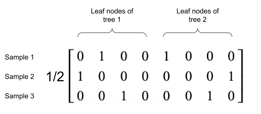 Figure 2 - An example Jacobian matrix for a random forest containing two decision trees, each with four leaf nodes.
We implemented a Seldonian random forest (SRF) model that uses scikit-learn's RandomForestClassifier as the initial model in this module. Here is the constructor of this class:
class SeldonianRandomForest(ClassificationModel):
    def __init__(self,**rf_kwargs):
        """ A Seldonian random forest model that re-labels leaf node probabilities
        from a vanilla decision tree built using SKLearn's RandomForestClassifier
        object.

        :ivar classifier: The SKLearn classifier object
        :ivar n_trees: The number of decision trees in the forest
        :ivar has_intercept: Whether the model has an intercept term
        :ivar params_updated: An internal flag used during the optimization
        """
        self.classifier = RandomForestClassifier(**rf_kwargs)
        self.n_trees = self.classifier.n_estimators
        self.has_intercept = False
        self.params_updated = False
Like the SeldonianDecisionTree model, the only inputs are the inputs you would normally provide to the scikit-learn RandomForestClassifier.
Note: If you are using a different library than scikit-learn for building the initial decision tree(s), you will need to carefully consider how to write down the Jacobian for your problem. This is also true if you using your own custom implementation, unless it is written purely in NumPy, SciPy and pure Python, in which case autograd will happily compute the Jacobian automatically.
Applying fair decision tree and random forest models to the GPA prediction problem from Tutorial E
We strongly encourage reading Tutorial E: Predicting student GPAs from application materials with fairness guarantees before proceeding here. In that tutorial, we created a Seldonian binary classifier and applied it to five different fairness constraints. The underlying ML model we used in that tutorial was a logistic regressor. In this section, we will compare the performance and safety properties of the Seldonian decision tree and Seldonian random forest models to the Seldonian logistic regressor as well as several baselines that do not consider the behavioral constraints.
Creating the specification object
There are a few differences between the script we used to create spec objects in Tutorial E and the one we will create here: i) the model object is now the SeldonianDecisionTree or SeldonianRandomForest model, ii) we use tighter versions of the same fairness constraints, and iii) we customize the hyperparameters of the KKT optimization. We used all of the default hyperparameters of the scikit-learn decision tree and random forest models except max_depth and n_estimators (for random forest). We chose a max_depth=5 to keep the model simple and to avoid overfitting, and we chose n_estimators=50 to get a reasonably-sized forest without incurring too much compute. In a real situation, one would tune these hyperparameters. Below is code snippet for creating the spec objects for each of the five fairness constraints from Tutorial E for the Seldonian decision tree model. Note that the data path and metadata path are local paths and must be adjusted to wherever you downloaded those two files. The two files can be downloaded from here.
import os
import autograd.numpy as np

from seldonian.dataset import DataSetLoader
from seldonian.parse_tree.parse_tree import make_parse_trees_from_constraints
from seldonian.utils.io_utils import save_pickle
from seldonian.spec import SupervisedSpec
from seldonian.models import objectives
from experiments.perf_eval_funcs import probabilistic_accuracy

from seldonian.models.trees.sktree_model import SeldonianDecisionTree, probs2theta

def initial_solution_fn(model,features,labels):
    probs = model.fit(features,labels)
    return probs2theta(probs)

if __name__ == "__main__":
    # 1. Dataset
    data_pth = '../../../../engine-repo-dev/static/datasets/supervised/GPA/gpa_classification_dataset.csv'
    metadata_pth = '../../../../engine-repo-dev/static/datasets/supervised/GPA/metadata_classification.json'
    regime='supervised_learning'
    sub_regime='classification'

    loader = DataSetLoader(
        regime=regime)
    dataset = loader.load_supervised_dataset(
        filename=data_pth,
        metadata_filename=metadata_pth,
        file_type='csv')
    all_feature_names = dataset.meta.feature_col_names
    sensitive_col_names = dataset.meta.sensitive_col_names
    frac_data_in_safety = 0.6

    # 2. Specify behavioral constraints
    deltas = [0.05] # confidence levels
    for constraint_name in ["disparate_impact",
        "demographic_parity","equalized_odds",
        "equal_opportunity","predictive_equality"]:
        # Define behavioral constraints
        if constraint_name == 'disparate_impact':
            epsilon = 0.9
            constraint_strs = [f'min((PR | [M])/(PR | [F]),(PR | [F])/(PR | [M])) >= {epsilon}']
        elif constraint_name == 'demographic_parity':
            epsilon = 0.1
            constraint_strs = [f'abs((PR | [M]) - (PR | [F])) <= {epsilon}']
        elif constraint_name == 'equalized_odds':
            epsilon = 0.15
            constraint_strs = [f'abs((FNR | [M]) - (FNR | [F])) + abs((FPR | [M]) - (FPR | [F])) <= {epsilon}']
        elif constraint_name == 'equal_opportunity':
            epsilon = 0.1
            constraint_strs = [f'abs((FNR | [M]) - (FNR | [F])) <= {epsilon}']
        elif constraint_name == 'predictive_equality':
            epsilon = 0.1
            constraint_strs = [f'abs((FPR | [M]) - (FPR | [F])) <= {epsilon}']

        parse_trees = make_parse_trees_from_constraints(
            constraint_strs,deltas,regime=regime,
            sub_regime=sub_regime,columns=sensitive_col_names)

        # 3. Define the underlying machine learning model
        max_depth = 5
        model = SeldonianDecisionTree(max_depth=max_depth)

        # 4. Create a spec object
        # Save spec object, using defaults where necessary
        spec = SupervisedSpec(
            dataset=dataset,
            model=model,
            parse_trees=parse_trees,
            sub_regime=sub_regime,
            frac_data_in_safety=frac_data_in_safety,
            primary_objective=objectives.Error_Rate,
            use_builtin_primary_gradient_fn=False,
            initial_solution_fn=initial_solution_fn,
            optimization_technique='gradient_descent',
            optimizer="adam",
            optimization_hyperparams={
                'lambda_init'   : np.array([0.5]),
                'alpha_theta'   : 0.005,
                'alpha_lamb'    : 0.005,
                'beta_velocity' : 0.9,
                'beta_rmsprop'  : 0.95,
                'use_batches'   : False,
                'num_iters'     : 800,
                'gradient_library': "autograd",
                'hyper_search'  : None,
                'verbose'       : True,
            }
        )
        os.makedirs('./specfiles',exist_ok=True)
        spec_save_name = f'specfiles/gpa_{constraint_name}_{epsilon}_fracsafety_{frac_data_in_safety}_sktree_maxdepth{max_depth}_reparam_spec.pkl'
        save_pickle(spec_save_name,spec,verbose=True)
Running this code will create fives specfiles in the directory: specfiles/. Next, we show how to create the five specfiles for the random forest model.
import os
import autograd.numpy as np

from seldonian.dataset import DataSetLoader
from seldonian.parse_tree.parse_tree import make_parse_trees_from_constraints
from seldonian.utils.io_utils import save_pickle
from seldonian.spec import SupervisedSpec
from seldonian.models import objectives
from experiments.perf_eval_funcs import probabilistic_accuracy

from seldonian.models.trees.skrandomforest_model import SeldonianRandomForest, probs2theta

def initial_solution_fn(model,features,labels):
    probs = model.fit(features,labels)
    return probs2theta(probs)

if __name__ == "__main__":
    # 1. Dataset
    data_pth = '../../../../../engine-repo-dev/static/datasets/supervised/GPA/gpa_classification_dataset.csv'
    metadata_pth = '../../../../../engine-repo-dev/static/datasets/supervised/GPA/metadata_classification.json'
    regime='supervised_learning'
    sub_regime='classification'

    loader = DataSetLoader(
        regime=regime)
    dataset = loader.load_supervised_dataset(
        filename=data_pth,
        metadata_filename=metadata_pth,
        file_type='csv')
    all_feature_names = dataset.meta.feature_col_names
    sensitive_col_names = dataset.meta.sensitive_col_names
    frac_data_in_safety = 0.6

    # 2. Specify behavioral constraints
    deltas = [0.05] # confidence levels
    for constraint_name in ["disparate_impact",
        "demographic_parity","equalized_odds",
        "equal_opportunity","predictive_equality"]:
        # Define behavioral constraints
        if constraint_name == 'disparate_impact':
            epsilon = 0.9
            constraint_strs = [f'min((PR | [M])/(PR | [F]),(PR | [F])/(PR | [M])) >= {epsilon}']
        elif constraint_name == 'demographic_parity':
            epsilon = 0.1
            constraint_strs = [f'abs((PR | [M]) - (PR | [F])) <= {epsilon}']
        elif constraint_name == 'equalized_odds':
            epsilon = 0.15
            constraint_strs = [f'abs((FNR | [M]) - (FNR | [F])) + abs((FPR | [M]) - (FPR | [F])) <= {epsilon}']
        elif constraint_name == 'equal_opportunity':
            epsilon = 0.1
            constraint_strs = [f'abs((FNR | [M]) - (FNR | [F])) <= {epsilon}']
        elif constraint_name == 'predictive_equality':
            epsilon = 0.1
            constraint_strs = [f'abs((FPR | [M]) - (FPR | [F])) <= {epsilon}']

        parse_trees = make_parse_trees_from_constraints(
            constraint_strs,deltas,regime=regime,
            sub_regime=sub_regime,columns=sensitive_col_names)

        # 3. Define the underlying machine learning model
        max_depth = 5
        n_estimators = 50
        model = SeldonianRandomForest(n_estimators=n_estimators,max_depth=max_depth)

        # 4. Create a spec object
        # Save spec object, using defaults where necessary
        spec = SupervisedSpec(
            dataset=dataset,
            model=model,
            parse_trees=parse_trees,
            sub_regime=sub_regime,
            frac_data_in_safety=frac_data_in_safety,
            primary_objective=objectives.Error_Rate,
            use_builtin_primary_gradient_fn=False,
            initial_solution_fn=initial_solution_fn,
            optimization_technique='gradient_descent',
            optimizer="adam",
            optimization_hyperparams={
                'lambda_init'   : np.array([0.5]),
                'alpha_theta'   : 0.005,
                'alpha_lamb'    : 0.005,
                'beta_velocity' : 0.9,
                'beta_rmsprop'  : 0.95,
                'use_batches'   : False,
                'num_iters'     : 800,
                'gradient_library': "autograd",
                'hyper_search'  : None,
                'verbose'       : True,
            }
        )
        os.makedirs('./specfiles',exist_ok=True)
        spec_save_name = f'specfiles/gpa_{constraint_name}_{epsilon}_fracsafety_{frac_data_in_safety}_skrf_maxdepth{max_depth}_{n_estimators}trees_reparam_spec.pkl'
        save_pickle(spec_save_name,spec,verbose=True)
This will save five more spec files to the specfiles/ directory. Now we will skip running the engine and go straight to running an experiment.
Running the Seldonian Experiments
Here we show a script for running the Seldonian experiment for the first constraint: disparate impact and for the Seldonian decision tree model only. Changing the script to run the experiments for the other constraints amounts to changing the constraint_name and epsilon variables. Changing the script to use the Seldonian random forest model amounts to changing the specfile variable.
The experiment will consist of 20 trials. This is fewer than we ran in Tutorial E, but it will be sufficient for comparing to the Seldonian logistic regressor and the baseline models. We will compare to three baseline models that do not consider the fairness constraints: i) a decision tree classifier trained with scikit-learn, ii) the same decision tree classifier as (i) but with leaf tuning using gradient descent, and iii) a logistic regressor trained with scikit-learn.
There are several minor differences between this tutorial and tutorial E that we want to point out here. Note that none of these affects the comparison between the models in this tutorial.
-
In this experiment, we omit the comparison to Fairlearn models, as that is not the purpose of this tutorial.
-
In this tutorial, we use a held-out test set of 1/3 of the original GPA dataset ($\sim$14,500 samples) for calculating the performance (left plot) and fairness violation (right plot). We resample the remaining 2/3 of the data ($\sim$28,800 samples) to make the trial datasets.
-
We use probabilistic accuracy rather than deterministic accuracy for the performance metric.
- We use the error rate (1-probabilistic accuracy) as the primary objective function, instead of the logistic loss as in Tutorial E.
Again, these differences do not affect the comparison between the Seldonian models because we use the same performance metrics and primary objectives for all models in this tutorial. We do not have control over the primary objective function used to fit the scikit-learn baselines, but we do evaluate them using the same performance metric as the Seldonian models.
import os
import numpy as np
from sklearn.model_selection import train_test_split

from seldonian.utils.io_utils import load_pickle
from seldonian.dataset import SupervisedDataSet
from seldonian.models.trees.sktree_model import probs2theta

from experiments.perf_eval_funcs import probabilistic_accuracy
from experiments.generate_plots import SupervisedPlotGenerator
from experiments.baselines.logistic_regression import BinaryLogisticRegressionBaseline
from experiments.baselines.random_classifiers import (
    UniformRandomClassifierBaseline,WeightedRandomClassifierBaseline)
from experiments.baselines.decision_tree import DecisionTreeClassifierBaseline
from experiments.baselines.random_forest import RandomForestClassifierBaseline
from experiments.baselines.decision_tree_leaf_tuning import DecisionTreeClassifierLeafTuningBaseline


def initial_solution_fn(model,features,labels):
    probs = model.fit(features,labels)
    return probs2theta(probs)

def perf_eval_fn(y_pred,y,**kwargs):
    return probabilistic_accuracy(y_pred,y)

def main():
    # Basic setup
    seed=4
    np.random.seed(seed)
    run_experiments = True
    make_plots = True
    save_plot = False
    include_legend = True
    frac_data_in_safety = 0.6

    model_label_dict = {
        'qsa':'Seldonian decision tree',
        'rf_qsa': 'Seldonian random forest (50 trees)',
        'logreg_qsa':'Seldonian logistic regressor',
        'decision_tree':'Sklearn decision tree (no constraint)',
        'decision_tree_leaf_tuning':'Sklearn decision tree with leaf tuning (no constraint)',
        'logistic_regression': 'Logistic regressor (no constraint)',
        } # also plot in this order
    # Change these to the fairness constraint of interest
    constraint_name = "disparate_impact"
    epsilon = 0.9

    # experiment parameters
    max_depth = 5
    performance_metric = '1 - error rate'
    n_trials = 20
    data_fracs = np.logspace(-4,0,15)
    n_workers = 6 # for parallel processing
    results_dir = f'results/sklearn_tree_testset0.33_{constraint_name}_{epsilon}_maxdepth{max_depth}_probaccuracy'
    plot_savename = os.path.join(results_dir,f'gpa_dtree_vs_logreg_{constraint_name}_{epsilon}.png')
    verbose=True

    # Load spec
    specfile = f'specfiles/gpa_{constraint_name}_{epsilon}_fracsafety_{frac_data_in_safety}_sktree_maxdepth{max_depth}_reparam_spec.pkl'
    spec = load_pickle(specfile)
    spec.initial_solution_fn = initial_solution_fn
    os.makedirs(results_dir,exist_ok=True)

    # Reset spec dataset to only use 2/3 of the original data,
    # use remaining 1/3 for ground truth set for the experiment
    # Use entire original dataset as ground truth for test set
    orig_features = spec.dataset.features
    orig_labels = spec.dataset.labels
    orig_sensitive_attrs = spec.dataset.sensitive_attrs
    # First, shuffle features
    (train_features,test_features,train_labels,
    test_labels,train_sensitive_attrs,
    test_sensitive_attrs
        ) = train_test_split(
            orig_features,
            orig_labels,
            orig_sensitive_attrs,
            shuffle=True,
            test_size=0.33,
            random_state=seed)

    new_dataset = SupervisedDataSet(
        features=train_features,
        labels=train_labels,
        sensitive_attrs=train_sensitive_attrs,
        num_datapoints=len(train_features),
        meta=spec.dataset.meta)

    # Set spec dataset to this new dataset
    spec.dataset = new_dataset
    # Setup performance evaluation function and kwargs

    perf_eval_kwargs = {
        'X':test_features,
        'y':test_labels,
        'performance_metric':performance_metric
        }

    plot_generator = SupervisedPlotGenerator(
        spec=spec,
        n_trials=n_trials,
        data_fracs=data_fracs,
        n_workers=n_workers,
        datagen_method='resample',
        perf_eval_fn=perf_eval_fn,
        constraint_eval_fns=[],
        results_dir=results_dir,
        perf_eval_kwargs=perf_eval_kwargs,
        )


    if run_experiments:
        # Baseline models
        lr_baseline = BinaryLogisticRegressionBaseline()
        plot_generator.run_baseline_experiment(
            baseline_model=lr_baseline,verbose=True)

        dt_classifier = DecisionTreeClassifierBaseline(max_depth=max_depth)
        plot_generator.run_baseline_experiment(
            baseline_model=dt_classifier,verbose=True)

        adam_kwargs={
        'n_iters_tot':350,
        'verbose': True,
        'debug': True
        }
        dt_leaf_tuning_baseline = DecisionTreeClassifierLeafTuningBaseline(
            primary_objective_fn=spec.primary_objective,sub_regime=spec.sub_regime,
            adam_kwargs=adam_kwargs,dt_kwargs={'max_depth':max_depth})
        plot_generator.run_baseline_experiment(
            baseline_model=dt_leaf_tuning_baseline,verbose=True)

        # Seldonian model
        plot_generator.run_seldonian_experiment(verbose=verbose)


    if make_plots:
        plot_generator.make_plots(fontsize=12,legend_fontsize=12,
            performance_label=performance_metric,
            ncols_legend=3,
            include_legend=include_legend,
            model_label_dict=model_label_dict,
            save_format="png",
            savename=plot_savename if save_plot else None)

if __name__ == "__main__":
    main()
In addition to running this script for the five fairness constraints for both Seldonian decision tree and Seldonian random forest, we also separately re-ran the experiments in Tutorial E using the same setup as these experiments (i.e., same constraints, performance metric, primary objective function, and held-out test set), so that we could compare the Seldonian decision tree, Seldonian random forest, and the Seldonian logistic regressor all on the same plots. The results from the five experiments are shown below. See the bottom row for the legend, which applies to all rows.
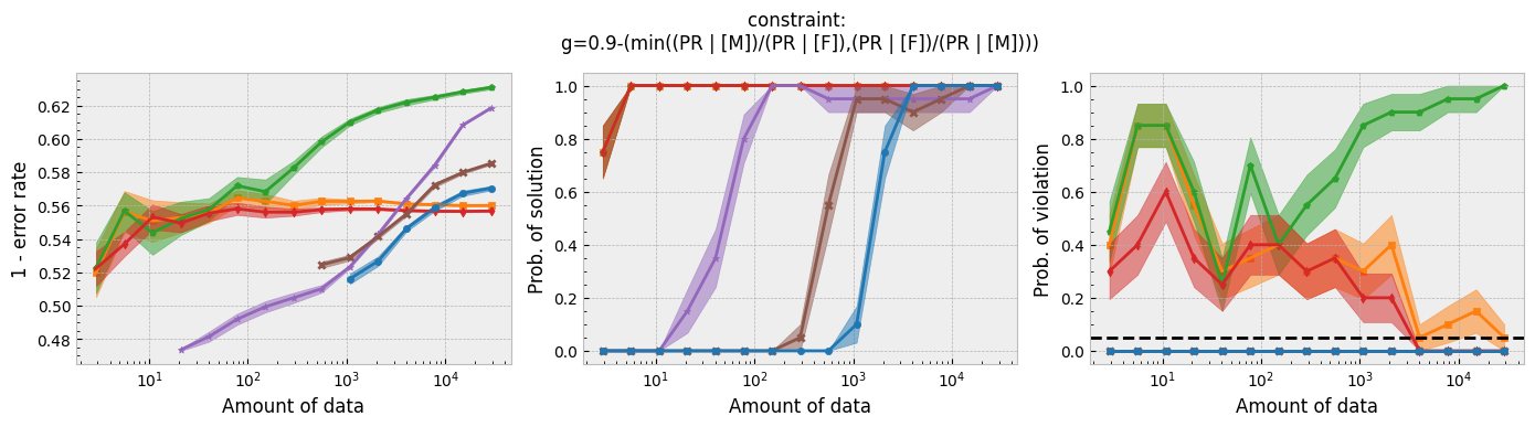
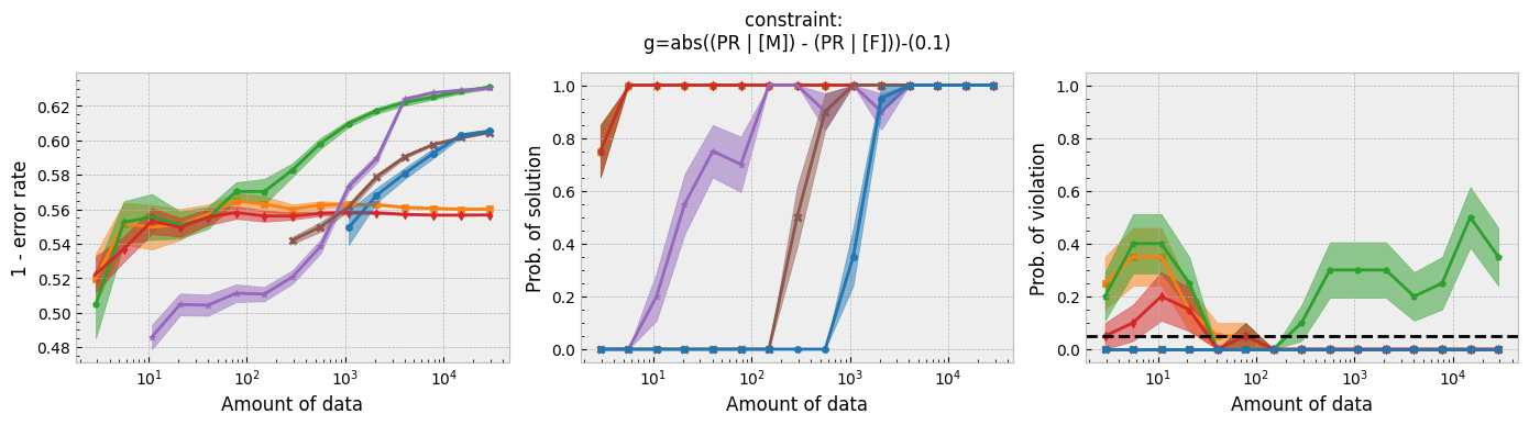
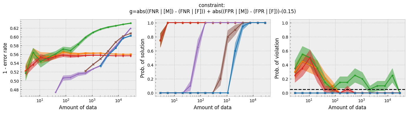
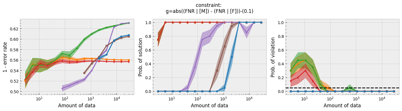
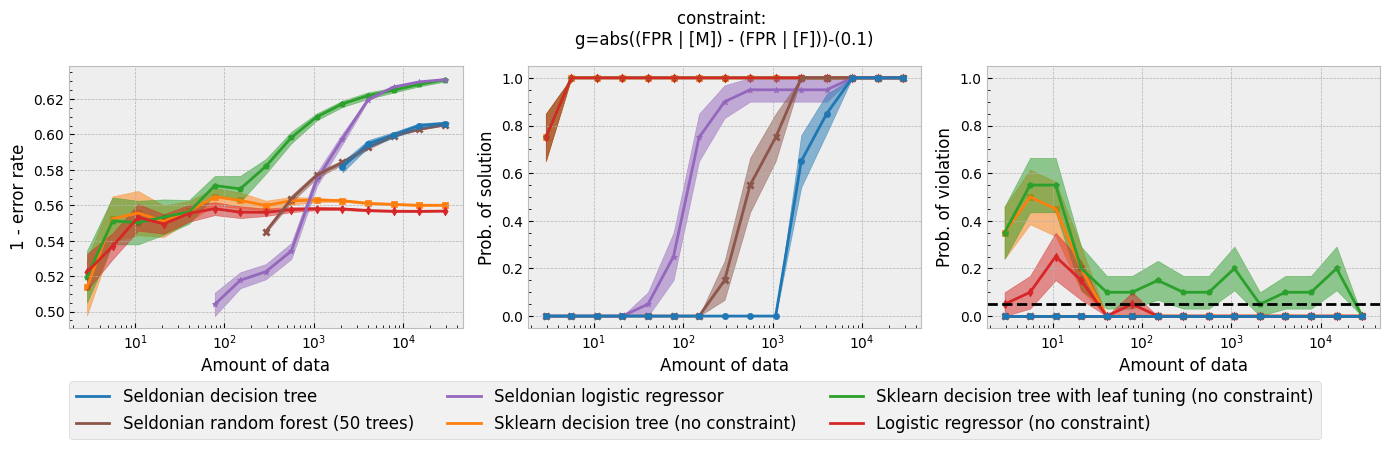 Figure 3 - Experiment plots for the GPA prediction problem for five fairness constraints. Each row of plots is an experiment for a different fairness constraint. From top to bottom: disparate impact, demographic parity, equalized odds, equal opportunity, and predictive equality. The Seldonian decision tree model (blue) and Seldonian random forest model (brown) are compared to the Seldonian logistic regressor (purple) discussed in Tutorial E and three baseline models trained without knowledge of the fairness constraints: i) a decision tree classifier trained with scikit-learn (orange), ii) the same decision tree classifier as (i) but with leaf tuning using gradient descent (green), and iii) a logistic regressor trained with scikit-learn (red). The colored points and bands in each panel show the mean and standard error over 20 trials, respectively.
Figure 3 shows that for all fairness constraints, the three Seldonian models have the desired behavior. That is, as the amount of data increases, their performance increases and the probability of returning a solution increases. Furthermore, they never violate the constraints. The Seldonian logistic regressor outperforms and returns solutions with less data than both of the tree-based Seldonian models. The Seldonian random forest generally performs as well or slightly better than the Seldonian decision tree and consistenly requires less data.
We included a new baseline in this tutorial for the first time which is now part of the toolkit: a decision tree classifier trained initially with scikit-learn, whose leaf node probabilities are then tuned using gradient descent (Figure 3; green). The purpose of this baseline is to provide a model that is as similar to the Seldonian tree-based models as possible, without considering the constraints. Figure 3 shows that this baseline achieves higher accuracy than the Seldonian decision tree, but it does this at the expense of being unfair, no matter the definition of fairness. The Seldonian logistic regressor achieves similar performance as this baseline for all constraints, and it is always fair, proving that accuracy does not need to be traded off with fairness for this problem.
Summary
In this tutorial, we introduced two tree-based models that can be trained to satisfy behavioral constraints with the Seldonian Toolkit. The first is a decision tree model (SDTree) which takes an initial decision tree trained with Scikit-Learn's DecisionTreeClassifier and tunes the leaf node label probabilities subject to fairness constraints using the toolkit's KKT-based optimization technique for candidate selection. We extend the basic SDTree model to a Seldonian random forest model, which takes an initial random forest trained with Scikit-Learn's RandomForestClassifier and, like in the single decision tree case, tunes the leaf node label probabilities of all trees in the forest. We provided our implementation of both of these models, but we stress that the technique can work regardless of the library or method used to create the initial decision tree or random forest. These techniques could also be extended to support other tree-based models such as boosted trees and other tree-bagging models. We encourange and support pull requests with new models, such as a new tree-based model.
We showed how to apply the Seldonian decision tree and Seldonian random forest models to an actual machine learning problem -- the GPA prediction problem with five fairness constraints from Tutorial E. Both models perform well and are always fair, with the random forest slightly outperforming and requiring less data to achieve fairness than the decision tree. The Seldonian logistic regressor from Tutorial E outperformed the Seldonian tree-based models. This is likely application-specific, and we are interested to see results applying Seldonian tree-based models to other problems.