Seldonian ML
GitHub
Tutorial H: Introduction to reinforcement learning with the Seldonian Toolkit
Contents
Introduction
The Seldonian Toolkit supports offline (batch) reinforcement learning (RL) Seldonian algorithms. In the RL setting, the user must provide data (the observations, actions, and rewards from past episodes), a policy parameterization (similar to a model in the supervised learning regime), and the desired behavioral constraints. Seldonian algorithms that are implemented via the engine search for a new policy that simultaneously optimizes a primary objective function (e.g., expected discounted return) and satisfies the behavioral constraints with high confidence. This tutorial builds on the previous supervised learning tutorials, so we suggest familiarizing yourself with those, in particular Tutorial C: Running the Seldonian Engine. Note that due to the choice of confidence-bound method used in this tutorial (Student's $t$-test), the algorithms in this tutorial are technically quasi-Seldonian algorithms (QSAs).
Outline
In this tutorial, after reviewing RL notation and fundamentals, you will learn how to:
- Define a RL Seldonian algorithm using data generated from a gridworld environment and a tabular softmax policy
- Run the algorithm using the Seldonian Engine to find a policy that satisfies a behavioral constraint
- Run a RL Seldonian Experiment for this Seldonian algorithm
RL background
In the RL regime, an agent interacts sequentially with an environment. Time is discretized into integer time steps $t \in \{0,1,2,\dotsc\}$. At each time step, the agent makes an observation $O_t$ about the current state $S_t$ of the environment. This observation can be noisy and incomplete. The agent then selects an action $A_t$, which causes the environment to transition to the next state $S_{t+1}$ and emit a scalar (real-valued) reward $R_t$. The agent's goal is to determine which actions will cause it to obtain as much reward as possible (we formalize this statement with math below).
Before continuing, we establish our notation for the RL regime:
- $t$: The current time step, starting at $t=0$.
- $S_t$: The state of the environment at time $t$.
- $O_t$: The agent's observation at time $t$. For many problems, the agent observes the entire state $S_t$. This can be accomplished by simply defining $O_t=S_t$.
- $A_t$: The action chosen by the agent at time $t$ (the agent selects $A_t$ after observing $O_t$).
- $R_t$: The reward received by the agent at time $t$ (the agent receives $R_t$ after the environment transitions to state $S_{t+1}$ due to action $A_t$).
- $\pi$: A policy, where $\pi(o,a)=\Pr(A_t=a|O_t=o)$ for all actions $a$ and observations $o$.
- $\pi_\theta$: A parameterized policy, which is simply a policy with a weight vector $\theta$ that changes the conditional distribution over $A_t$ given $O_t$. That is, for all actions $a$, observations $o$, and weight vectors $\theta$, $\pi_\theta(o,a) = \Pr(A_t=a|O_t=o ; \theta)$, where "$;\theta$" indicates "given that the agent uses policy parameters $\theta$". This is not quite the same as a conditional probability because $\theta$ is not an event (one should not apply Bayes' theorem to this expression thinking that $\theta$ is an event).
- $\gamma$: The reward discount parameter. This is a problem-specific constant in $[0,1]$ that is used in the objective function, defined next.
- $J$: The objective function. The default in the toolkit is the expected discounted return: $J(\pi)=\mathbf{E}\left [ \sum_{t=0}^\infty \gamma^t R_t\right ]$. The agent's goal is to find a policy that maximizes this objective function.
- The agent's experiences can be broken into statistically independent episodes. Each episode begins at time $t=0$. When an episode ends, the agent no longer needs to select actions and no longer receives rewards (this can be modeled using a terminal absorbing state as defined on page 18 here).
At this time, the Seldonian Toolkit is only compatible with batch or offline RL. This means that some current policy (typically called the behavior policy $\pi_b$) is already in use to select actions. The available data corresponds to the observations, actions, and rewards from previous episodes wherein the current policy was used. To make this more formal, we will define a history $H$ to be the available historical information from one episode:
$$ H = (O_0, A_0, R_0, O_1, A_1, R_1, \dotsc).$$
All of the available data can then be expressed as $D = (H_i)_{i=1}^m$, where $m$ is the number of episodes for which data is available.
For generality, the toolkit does not require there to be just one current policy. Instead, the available data could have been generated by several different (past) policies. However, the default Seldonian RL algorithms in the toolkit require some knowledge about what the past policies were. Specifically, they require each action $A_t$ in the historical data to also come with the probability that the behavior policy (the policy that selected the action) would select that action: $\pi_b(O_t,A_t)$. Hence, we amend the definition of a history $H$ to include this information:
$$ H = (O_0, A_0, \pi_b(O_0,A_0), R_0, O_1, A_1, \pi_b(O_1,A_1) R_1, \dotsc).$$
Notice that in this batch setting, Seldonian RL algorithms can be used to improve upon current and past policies. However, they can't be used to construct the first policy for an application.
Define the environment and policy
The first steps in setting up an RL Seldonian algorithm are to select an environment of interest and then to specify the policy parameterization the agent should use. That is, how does $\theta$ change the policy $\pi_\theta$? For example, when using a neural network as the policy, this corresponds to determining the network architecture and how the network's outputs specify the probability of each possible action.
Defining the environment
In this tutorial, we will consider a 3x3 gridworld environment as shown in the figure below.
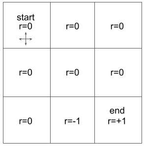 Figure 1 – A 3x3 gridworld where the initial state ($S_0$) is the upper left cell. Episodes end when the agent reaches the bottom right cell, which we refer to as the "terminal state." This problem is fully observable, meaning that the agent observes the entire state, $O_t=S_t$, always. The possible actions are up, down, left, and right, which cause the agent to move one cell in the specified direction. Hitting a wall, e.g., action=left in the initial state, is a valid action and returns the agent to the same state, i.e., $S_{t+1}=S_t$. Each cell is labeled with the reward that the agent receives when that state is $S_{t+1}$. For example, if the agent transitions from the middle state ($S_t$) to the bottom middle state ($S_{t+1}$) then the reward would be $R_t=-1$. Notice that the reward is $0$ in all cells except for a $-1$ reward in the bottom middle cell and a $+1$ reward when reaching the terminal state. We will use a discount factor of $\gamma=0.9$ for this environment when calculating the expected return of a policy.
Defining the policy
The toolkit is compatible with a wide range of possible policy parameterizations, and even allows you to introduce your own environment-specific policy representation. For this example, we will use a tabular softmax policy. This policy stores one policy parameter (weight) for every possible observation-action pair. Let $\theta_{o,a}$ be the parameter for observation $o$ and action $a$. A tabular softmax policy can then be expressed as:
$$ \begin{equation}
\pi_\theta(o,a) = \frac{e^{\theta_{o,a}}}{\sum_{a'}{e^{\theta_{o,a'}}}}
\label{policy_parameterization}
\end{equation}
$$
So, given the current observation $O_t$, the agent chooses an action by drawing from a discrete probability distribution where the probability of each action $a$ is $\pi(O_t,a)$.
Consider the offline RL problem of finding a policy for the 3x3 gridworld that has the largest expected return possible (primary objective) subject to the safety constraint that the expected return is at least $-0.25$ (this might be the performance of the current policy). In this tutorial, we simulate this process, generating many episodes of data using a behavior policy (current policy) and then feeding this data to our Seldonian algorithm with the tabular softmax policy parameterization. We include a behavioral constraint that requires the performance of the new policy to be at least $-0.25$ with probability at least $0.95$. In later tutorials, we show how safety constraints can be defined in terms of additional reward functions (as in constrained Markov decision processes [MDPs]).
For those familiar with off-policy evaluation (OPE), our algorithms use off-policy estimates of the expected return based on various importance sampling estimators. These estimates are used both in the primary objective (to maximize the expected discounted return) and sometimes in safety constraints (like in this example, where the safety constraint requires the performance of the new policy to be at least $-0.25$). In this tutorial, we will use the ordinary importance sampling estimator, which provides unbiased estimates of $J(\pi_\theta)$, for any $\theta$. These unbiased estimates are used like the unbiased estimates $\hat g$ and $\hat z$ described in the tutorials for the supervised learning regime.
In summary, we will apply a Seldonian RL algorithm to ensure that the performance of the new policy is at least the performance of the behavior policy $(-0.25)$, with probability at least $0.95$. The algorithm will use 1,000 episodes of data generated using the behavior policy (which selects each action with equal probability). We selected the performance threshold of $-0.25$ by running 10,000 additional episodes using the behavior policy and computing the average discounted return, giving $J(\pi_b)\approx -0.25$. We can now write out the Seldonian ML problem:
Find a new policy subject to the constraint:
- $g1: \text{J_pi_new_IS} \geq -0.25$, and $\delta=0.05$
where $\text{J_pi_new_IS}$ is an RL-specific
measure function, which means that the engine is programmed to interpret $\text{J_pi_new_IS}$ as the performance of the new policy, as evaluated using ordinary importance sampling with data generated by the behavior policy. Other importance sampling estimators can be referenced via different suffixes, such as $\text{J_pi_new_PDIS}$ for per-decision importance sampling.
From supervised learning to reinforcement learning
From the toolkit's perspective, there are few differences between the supervised learning and reinforcement learning regimes. The algorithm overview remains unchanged: the Seldonian algorithm still has candidate selection and safety test modules. It still uses gradient descent using the KKT conditions (or black box optimization) to find the candidate solutions and uses statistical tools like Student's $t$-test to compute confidence intervals. Though there are some differences in the code (as shown in the example below), the core conceptual differences are:
- The parameterized "model" is replaced with a parameterized "policy." However, this is mostly just a terminology change (both take an input and provide a distribution over possible outputs).
- Though both still use a parse tree to represent the behavioral constraints, in the RL regime the base variables (leaf nodes of the parse tree that are not constants) use importance sampling variants to estimate what would happen if a new policy were to be used. More precisely, they provide unbiased estimates of the expected discounted return of the new policy, and this expected discounted return can use additional rewards defined to capture the safety of the new policy. The importance sampling estimates correspond to the $\hat z$ functions described in the Algorithm details tutorial.
- The data consist of $m$ episodes in the RL regime as opposed to $m$ data points in the supervised learning regime.
- In the Experiments library, the default way of generating ground truth data in the RL regime is to run additional episodes using a behavior policy. We will see this played out in the Running a Seldonian Experiment section.
Creating the specification object
Our goal is to create an RLSpec object (analogous to the SupervisedSpec object), which will consist of everything we will need to run a Seldonian algorithm using the engine. Creating this object involves defining the behavior dataset, policy parameterization, any environment-specific parameters, and the behavioral constraints.
In general, the manner in which the behavior data is generated is not important. In fact, generating data is not something a user will typically do using the engine. However, for this tutorial, we will generate synthetic data for reproducibility purposes. The data file we will create can be found here if you would like to skip this step: gridworld_1000episodes.pkl. We will use the Gridworld environment that is part of the Engine library. This Python class implements a generalized version of the gridworld environment described in Figure 1. It defines a square gridworld of arbitrary size, where the default size and reward function match the description in Figure 1. Therefore, we can use this environment without modification. We will use an agent that adopts a uniform random softmax policy. The weights of the policy are used to generate the action probabilities as in equation \eqref{policy_parameterization}. Because there are 9 states and 4 possible actions, there are a total of 36 weights. The behavior policy sets all of these weights to zero, such that the probability of each action after any observation is $p=0.25$, i.e., uniform random.
We will use the run_trial() in the RL_runner module to generate the data. A trial is a set of episodes. This function takes as input a dictionary where we provide the specification of the trial, such as the number of episodes, a function to create the environment, and a function to create the agent. The reason we provide functions to create the environment and agent instead of those objects themselves is so that we can create new instances of those objects in parallel processes to speed up the data generation process. Again, this step is only necessary for generating the data, which users will either not need to do or will potentially do outside of the Engine library.
Save this script as a file called generate_data.py and run it from the command line like
$ python generate_data.py
This saves a file called gridworld_1000episodes.pkl in the current directory which contains the 1000 episodes.
Now we can use these episodes to create a RLDataSet object and complete the spec file. We will use the createRLSpec() function which takes as input a dataset, policy, constraint strings, deltas, and environment-specific keyword arguments. This function hides some defaults to the RLSpec object for convenience here. The dataset will be created from the episodes we just saved in one line. We already specified our constraint strings and deltas above.
We create a custom policy class called GridworldSoftmaxwhich inherits from the DiscreteSoftmax base class. The "discrete" in the name comes from the fact that the observation space and the action space are both discrete-valued, as opposed to continuous-valued. We use a custom class to i) show how to subclass a policy base class and ii) speed up the computation of action probabilities given (observation,action) pairs. The DiscreteSoftmax base class does not assume that observations and actions are provided in 0-indexed form, so before it evaluates the action probabilities, it transforms them to 0-indexed form. In our case, we generated behavior data where the observations and actions are 0-indexed, so we can take advantage of that to speed up our code. This will be particularly helpful when we run an experiment below, which calls the engine many times. Note the signature of the method: get_probs_from_observations_and_actions(self,observations,actions,_). This is a method that every policy class must have, and it takes three arguments: observations,actions,behavior_action_probs. In our case, we don't use the behavior action probabilities, so we use the placeholder _ for that parameter.
The policy requires some knowledge of the environment, which we call a Env_Description. This is just a description of the observation and action spaces, which we define as objects. In our case, the only additional environment-specific piece of information is the discount factor, $\gamma=0.9$, which we specify in the env_kwargs argument.
# createSpec.py
import autograd.numpy as np
from seldonian.RL.Agents.Policies.Softmax import DiscreteSoftmax
from seldonian.RL.Env_Description.Env_Description import Env_Description
from seldonian.RL.Env_Description.Spaces import Discrete_Space
from seldonian.spec import createRLSpec
from seldonian.dataset import RLDataSet,RLMetaData
from seldonian.utils.io_utils import load_pickle

class GridworldSoftmax(DiscreteSoftmax):
    def __init__(self, env_description):
        hyperparam_and_setting_dict = {}
        super().__init__(hyperparam_and_setting_dict, env_description)

    def get_probs_from_observations_and_actions(self,observations,actions,_):
        return self.softmax(self.FA.weights)[observations,actions]

    def softmax(self,x):
        e_x = np.exp(x - np.max(x, axis=1, keepdims=True))
        return e_x / e_x.sum(axis=1, keepdims=True)

def main():
    episodes_file = './gridworld_1000episodes.pkl'
    episodes = load_pickle(episodes_file)
    meta = RLMetaData(all_col_names=["episode_index", "O", "A", "R", "pi_b"])
    dataset = RLDataSet(episodes=episodes,meta=meta)

    # Initialize policy
    num_states = 9
    observation_space = Discrete_Space(0, num_states-1)
    action_space = Discrete_Space(0, 3)
    env_description =  Env_Description(observation_space, action_space)
    policy = GridworldSoftmax(env_description=env_description)
    env_kwargs={'gamma':0.9}
    save_dir = '.'
    constraint_strs = ['J_pi_new_IS >= -0.25']
    deltas=[0.05]

    spec = createRLSpec(
        dataset=dataset,
        policy=policy,
        constraint_strs=constraint_strs,
        deltas=deltas,
        env_kwargs=env_kwargs,
        save=True,
        save_dir='.',
        verbose=True)

if __name__ == '__main__':
    main()
Saving this script to a file called createSpec.py and then running it the command line like:
$ python createSpec.py
will create a file called spec.pkl in whatever directory you ran the command. Once that file is created, you are ready to run the Seldonian algorithm.
Running the Seldonian Engine
Now that we have the spec file, running the Seldonian algorithm is simple. You may need to change the path to specfile if your spec file is saved in a location other than the current directory. We will also change some of the defaults of the optimization process; namely, we will set the number of iterations to $10$ and set the learning rates of $\theta$ and $\lambda$ to $0.01$.
This should result in the following output, though the exact numbers may differ due to your machine's random number generator:
Safety dataset has 600 episodes
Candidate dataset has 400 episodes
Have 10 epochs and 1 batches of size 400 for a total of 10 iterations
Epoch: 0, batch iteration 0
Epoch: 1, batch iteration 0
Epoch: 2, batch iteration 0
Epoch: 3, batch iteration 0
Epoch: 4, batch iteration 0
Epoch: 5, batch iteration 0
Epoch: 6, batch iteration 0
Epoch: 7, batch iteration 0
Epoch: 8, batch iteration 0
Epoch: 9, batch iteration 0
Passed safety test!
The solution found is:
[[ 0.20093676  0.20021209 -0.20095315  0.2018718 ]
 [ 0.19958715  0.21193489 -0.21250555 -0.20173669]
 [ 0.20076256 -0.19977755  0.21200753 -0.20160111]
 [ 0.20127782  0.21320971 -0.20111709  0.19984976]
 [ 0.19655251  0.20152484 -0.20126941 -0.19943337]
 [-0.20448104 -0.2002143   0.20163945 -0.20272628]
 [ 0.20233235 -0.20099993  0.20002241  0.20128514]
 [ 0.20062167  0.20107532 -0.20115979 -0.20080426]
 [ 0.          0.          0.          0.        ]]
As we can see, the solution returned by candidate selection passed the safety test. The solution shows the weights $\theta(s,a)$ of the new policy, where the $j$th column in the $i$th row represents the $j$th action given the $i$th observation (also state, in this case) in the gridworld. The final row is all zeros because no actions are taken from the terminal state. This may not be a particularly good solution, but we have a high-probability guarantee that it is better than the uniform random policy.
Running a Seldonian Experiment
Now that we have successfully run the Seldonian algorithm once with the engine, we are ready to run a Seldonian Experiment. This will help us better understand the safety and performance of our new policies. It will also help us understand how much data we need to meet the safety and performance requirements of our problem. We recommend reading the Experiments overview before continuing here. If you have not already installed the Experiments library, follow the instructions here to do so.
Here is an outline of the experiment we will run:
-
Create an array of data fractions, which will determine how much of the data to use as input to the Seldonian algorithm in each trial. We will use 10 different data fractions, which will be log-spaced between approximately 0.005 and 1.0. This array times the number of episodes in the original dataset (1,000) will make up the horizontal axis of the three plots, i.e., the "amount of data."
-
Create 20 datasets (one for each trial) by rerunning the behavior data generation process with a different random seed. Each regenerated dataset will have the same number of episodes (1,000) as the original dataset. We use 20 trials so that we can compute uncertainties on the plotted quantities at each data fraction.
-
For each
data_frac in the array of data fractions, run 20 trials. This will result in 200 total trials. In each trial:
-
Use only the first
data_frac fraction of episodes from the corresponding trial dataset to run the Seldonian algorithm using the Seldonian Engine.
-
If the safety test passes, return the new policy parameters obtained via the Seldonian algorithm. If not, return "NSF" for no solution found.
-
If the safety test passes, generate 1,000 episodes using the new policy parameters. This is data set on which the performance and safety metrics will be calculated for this trial.
-
For each
data_frac, calculate the mean and standard error on the performance (expected discounted return) across the 20 trials at this data_frac. This will be the data used for the first of the three plots. Also record how often a solution was returned and passed the safety test across the 20 trials. This fraction, referred to as the "solution rate," will be used to make the second of the three plots. Finally, for the trials that returned solutions that passed the safety test, calculate the fraction of trials for which the constraint was violated on the ground truth episodes. The fraction violated will be referred to as the "failure rate" and will make up the third and final plot.
Now, we will show how to implement the described experiment using the Experiments library. At the center of the Experiments library is the PlotGenerator class, and in our particular example, the RLPlotGenerator child class. The goal of the following script is to set up this object, use its methods to run our experiments, and then to make the three plots.
First, the necessary imports:
# run_experiment.py
from functools import partial
import os
os.environ["OMP_NUM_THREADS"] = "1"
import autograd.numpy as np   # Thinly-wrapped version of Numpy
from concurrent.futures import ProcessPoolExecutor

from seldonian.utils.io_utils import load_pickle
from seldonian.utils.stats_utils import weighted_sum_gamma
from seldonian.RL.RL_runner import run_episode
from seldonian.RL.environments.gridworld import Gridworld
from seldonian.RL.Agents.Parameterized_non_learning_softmax_agent import Parameterized_non_learning_softmax_agent

from experiments.generate_plots import RLPlotGenerator

from createSpec import GridworldSoftmax
The line os.environ["OMP_NUM_THREADS"] = "1" in the imports block above turns off NumPy's implicit parallelization, which we want to do when using n_workers>1 (see Tutorial M: Efficient parallelization with the toolkit for more details).
Now, we will define functions for creating the environment and agent (these are the same as the ones in generate_data.py), and the function for evaluating the performance. The latter function takes as input keyword arguments containing the model and the number of episodes we are using for evaluation. This function returns both the generated episodes and the discounted expected return.
def generate_episodes_and_calc_J(**kwargs):
    """ Calculate the expected discounted return
    by generating episodes under the new policy

    :return: episodes, J, where episodes is the list
        of generated ground truth episodes and J is
        the expected discounted return
    :rtype: (List(Episode),float)
    """
    model = kwargs['model']
    num_episodes = kwargs['n_episodes_for_eval']
    hyperparameter_and_setting_dict = kwargs['hyperparameter_and_setting_dict']

    # Get trained model weights from running the Seldonian algo
    new_params = model.policy.get_params()

    # Create the env and agent (setting the new policy params)
    # and run the episodes
    episodes = []
    env = create_env_func()
    agent = create_agent_func(new_params)
    for i in range(num_episodes):
        episodes.append(run_episode(agent,env))

    # Calculate J, the discounted sum of rewards
    returns = np.array([weighted_sum_gamma(ep.rewards,gamma=0.9) for ep in episodes])
    J = np.mean(returns)
    return episodes,J
Next, we set up the parameters for the experiments, such as the data fractions we want to use and how many trials at each data fraction we want to run. Each trial in an experiment is independent of all other trials, so parallelization can speed experiments up enormously. Set n_workers to however many CPUs you want to use (again, see Tutorial M: Efficient parallelization with the toolkit for more details). The results for each experiment we run will be saved in subdirectories of results_dir. Change this variable as desired. n_episodes_for_eval determines how many episodes are used for evaluating the performance and failure rate.
if __name__ == "__main__":
    # Parameter setup
    run_experiments = True
    make_plots = True
    save_plot = False
    performance_metric = 'J(pi_new)'
    n_trials = 20
    data_fracs = np.logspace(-2.3,0,10)
    n_workers = 8
    verbose=True
    results_dir = f'results/gridworld_tutorial'
    os.makedirs(results_dir,exist_ok=True)
    plot_savename = os.path.join(results_dir,f'gridworld_{n_trials}trials.png')
    n_episodes_for_eval = 1000
We will need to load the same spec object that we created for running the engine. As before, change the path to where you saved this file. We will modify some of the hyperparameters of gradient descent. This is not necessary, but we found that using these parameters resulted in better performance than the default parameters that we used to run the engine a single time. This also illustrates how to modify the spec object before running an experiment, which can be useful.
    # Load spec
    specfile = './spec.pkl'
    spec = load_pickle(specfile)
    spec.optimization_hyperparams['num_iters'] = 40
    spec.optimization_hyperparams['alpha_theta'] = 0.01
    spec.optimization_hyperparams['alpha_lamb'] = 0.01
One of the remaining parameters of the plot generator is perf_eval_fn, a function that will be used to evaluate the performance in each trial. In general, this function is completely up to the user to define. During each trial, this function is called after the Seldonian algorithm has been run and only if the safety test passed for that trial. The kwargs passed to this function will always consist of the model object from the current trial and the hyperparameter_and_setting_dict. There is also the option to pass additional keyword arguments to this function via the perf_eval_kwargs parameter.
We will write this function to generate 1000 episodes using the policy obtained by running the Seldonian algorithm and calculate the expected discounted return (with $\gamma = 0.9$). The only additional kwarg we need to provide is how many episodes to run. In this function, we create a fresh gridworld environment and agent so these are independent across trials. We set the agent's weights to the weights that were trained by the Seldonian algorithm so that the data are generated using the new policy obtained by the Seldonian algorithm.
    def generate_episodes_and_calc_J(**kwargs):
        """ Calculate the expected discounted return
        by generating episodes

        :return: episodes, J, where episodes is the list
            of generated ground truth episodes and J is
            the expected discounted return
        :rtype: (List(Episode),float)
        """
        # Get trained model weights from running the Seldonian algo
        model = kwargs['model']
        new_params = model.policy.get_params()

        # create env and agent
        hyperparameter_and_setting_dict = kwargs['hyperparameter_and_setting_dict']
        agent = create_agent_fromdict(hyperparameter_and_setting_dict)
        env = Gridworld(size=3)

        # set agent's weights to the trained model weights
        agent.set_new_params(new_params)

        # generate episodes
        num_episodes = kwargs['n_episodes_for_eval']
        episodes = run_trial_given_agent_and_env(
            agent=agent,env=env,num_episodes=num_episodes)

        # Calculate J, the discounted sum of rewards
        returns = np.array([weighted_sum_gamma(ep.rewards,env.gamma) for ep in episodes])
        J = np.mean(returns)
        return episodes,J
    perf_eval_kwargs = {'n_episodes_for_eval':n_episodes_for_eval}
Next, we need to define the hyperparameter_and_setting_dict as we did in the createSpec.py script above. This is required for generating the datasets that we will use in each of the 20 trials, as well as for generating the data in the function we defined to evaluate the performance. Note that in this case the number of episodes that we use for generating the trial datasets and the number of episodes that we use for evaluating the performance are the same. This does not need to be the case, as we can pass a different value for n_episodes_for_eval via perf_eval_kwargs if we wanted to.
    hyperparameter_and_setting_dict = {}
    hyperparameter_and_setting_dict["env"] = Gridworld(size=3)
    hyperparameter_and_setting_dict["agent"] = "Parameterized_non_learning_softmax_agent"
    hyperparameter_and_setting_dict["num_episodes"] = 1000
    hyperparameter_and_setting_dict["num_trials"] = 1
    hyperparameter_and_setting_dict["vis"] = False
Now we are ready to make the RLPlotGenerator object.
    plot_generator = RLPlotGenerator(
        spec=spec,
        n_trials=n_trials,
        data_fracs=data_fracs,
        n_workers=n_workers,
        datagen_method='generate_episodes',
        hyperparameter_and_setting_dict=hyperparameter_and_setting_dict,
        perf_eval_fn=perf_eval_fn,
        perf_eval_kwargs=perf_eval_kwargs,
        results_dir=results_dir,
        )
To run the experiment, we simply run the following code block:
    if run_experiments:
        plot_generator.run_seldonian_experiment(verbose=verbose)
After the experiment is done running, we can make the three plots, which is done in the following code block:
    if make_plots:
        plot_generator.make_plots(
            fontsize=12,
            legend_fontsize=12,
            performance_label=performance_metric,
            savename=plot_savename if save_plot else None,
            save_format="png")
Here is the entire script, saved in a file called generate_gridworld_plots.py. We put the function definition for evaluating the performance outside of the main block in the full script for clarity. This is a slightly different place than where we presented it in the step-by-step code blocks above.
# run_experiment.py
from functools import partial
import os
os.environ["OMP_NUM_THREADS"] = "1"
import autograd.numpy as np   # Thinly-wrapped version of Numpy
from concurrent.futures import ProcessPoolExecutor

from seldonian.utils.io_utils import load_pickle
from seldonian.utils.stats_utils import weighted_sum_gamma
from seldonian.RL.RL_runner import run_episode
from seldonian.RL.environments.gridworld import Gridworld
from seldonian.RL.Agents.Parameterized_non_learning_softmax_agent import Parameterized_non_learning_softmax_agent

from experiments.generate_plots import RLPlotGenerator

from createSpec import GridworldSoftmax

def create_env_func():
    return Gridworld(size=3)

def create_agent_func(new_params):
    dummy_env = Gridworld(size=3)
    env_description = dummy_env.get_env_description()
    agent = Parameterized_non_learning_softmax_agent(
        env_description=env_description,
        hyperparam_and_setting_dict={},
    )
    agent.set_new_params(new_params)
    return agent

def generate_episodes_and_calc_J(**kwargs):
    """ Calculate the expected discounted return
    by generating episodes

    :return: episodes, J, where episodes is the list
        of generated ground truth episodes and J is
        the expected discounted return
    :rtype: (List(Episode),float)
    """
    model = kwargs['model']
    num_episodes = kwargs['n_episodes_for_eval']
    hyperparameter_and_setting_dict = kwargs['hyperparameter_and_setting_dict']

    # Get trained model weights from running the Seldonian algo
    new_params = model.policy.get_params()

    # Create the env and agent (setting the new policy params)
    # and run the episodes
    episodes = []
    env = create_env_func()
    agent = create_agent_func(new_params)
    for i in range(num_episodes):
        episodes.append(run_episode(agent,env))

    # Calculate J, the discounted sum of rewards
    returns = np.array([weighted_sum_gamma(ep.rewards,gamma=0.9) for ep in episodes])
    J = np.mean(returns)
    return episodes,J

if __name__ == "__main__":
    # Parameter setup
    np.random.seed(99)
    run_experiments = True
    make_plots = True
    save_plot = False
    include_legend = True

    num_episodes = 1000 # For making trial datasets and for looking up specfile
    n_episodes_for_eval = 1000
    n_trials = 20
    data_fracs = np.logspace(-3,0,10)
    n_workers_for_episode_generation = 1
    n_workers = 6

    frac_data_in_safety = 0.6
    verbose=True
    results_dir = f'results/gridworld_{num_episodes}episodes_{n_trials}trials'
    os.makedirs(results_dir,exist_ok=True)
    plot_savename = os.path.join(results_dir,f'gridworld_experiment.png')
    # Load spec
    specfile = f'./spec.pkl'
    spec = load_pickle(specfile)

    perf_eval_fn = generate_episodes_and_calc_J
    perf_eval_kwargs = {
        'n_episodes_for_eval':n_episodes_for_eval,
        'env_kwargs':spec.model.env_kwargs,
    }
    initial_solution = np.zeros((9,4)) # theta values
    # The setup for generating behavior data for the experiment trials.
    hyperparameter_and_setting_dict = {}
    hyperparameter_and_setting_dict["create_env_func"] = create_env_func
    hyperparameter_and_setting_dict["create_agent_func"] = partial(
        create_agent_func,
        new_params=initial_solution,
    )
    hyperparameter_and_setting_dict["num_episodes"] = num_episodes
    hyperparameter_and_setting_dict["n_workers_for_episode_generation"] = n_workers_for_episode_generation
    hyperparameter_and_setting_dict["num_trials"] = 1 # Leave as 1 - it is not the same "trial" as experiment trial.
    hyperparameter_and_setting_dict["vis"] = False

    plot_generator = RLPlotGenerator(
        spec=spec,
        n_trials=n_trials,
        data_fracs=data_fracs,
        n_workers=n_workers,
        datagen_method='generate_episodes',
        hyperparameter_and_setting_dict=hyperparameter_and_setting_dict,
        perf_eval_fn=perf_eval_fn,
        perf_eval_kwargs=perf_eval_kwargs,
        results_dir=results_dir,
        )

    if run_experiments:
        plot_generator.run_seldonian_experiment(verbose=verbose)

    if make_plots:
        plot_generator.make_plots(fontsize=18,
            performance_label=r"$J(\pi_{\mathrm{new}})$",
            include_legend=include_legend,
            save_format="png",
            title_fontsize=18,
            legend_fontsize=16,
            custom_title=r"$J(\pi_{\mathrm{new}}) \geq -0.25$ (vanilla gridworld 3x3)",
            savename=plot_savename if save_plot else None)
Running the script should produce a plot that looks very similar to the one below. Once the experiments are run, if you want to save the plot but not rerun the experiments simply set: run_experiments = False and save_plot = True.
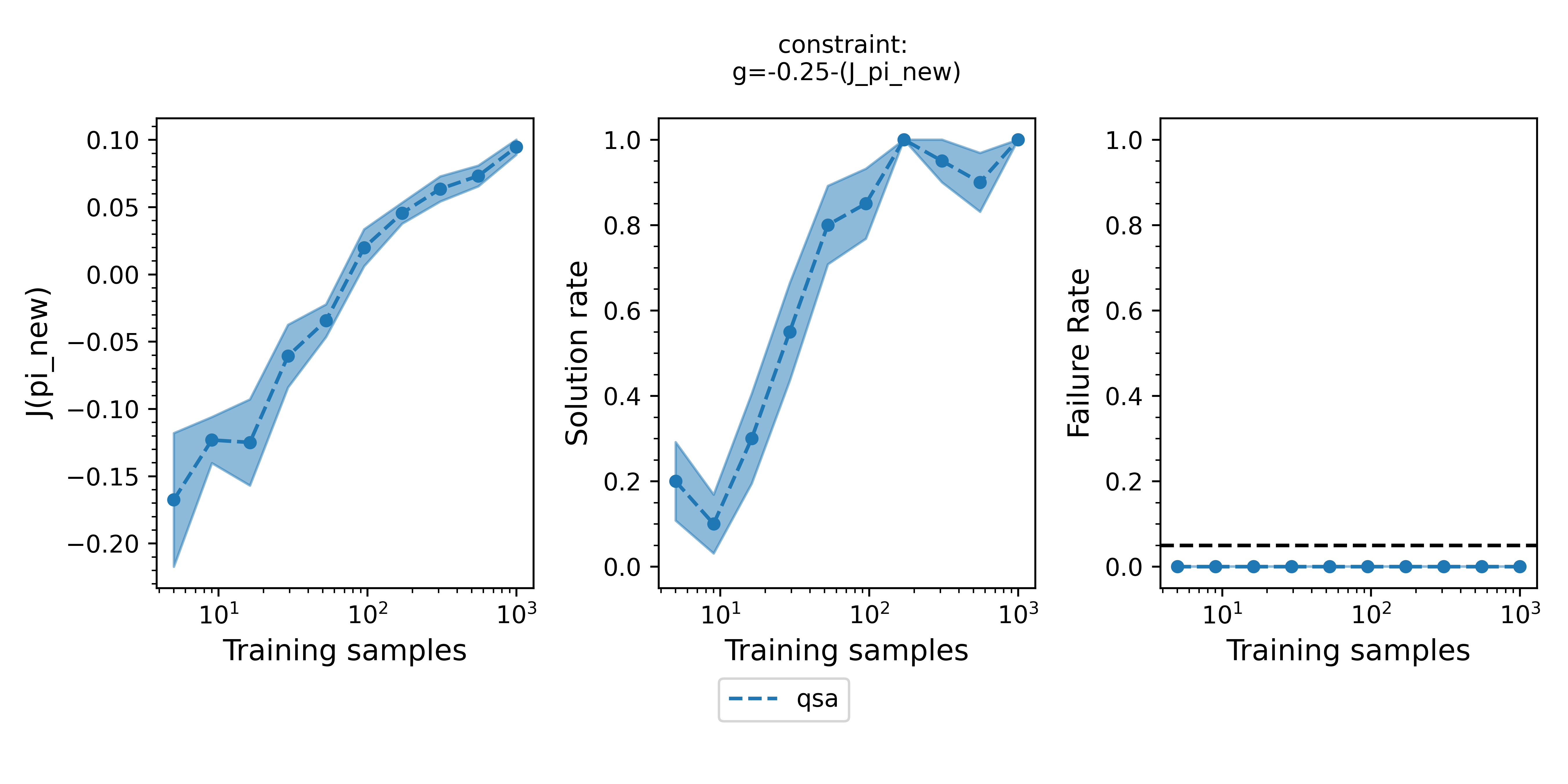 Figure 2 - The three plots of a Seldonian Experiment shown for the gridworld environment with a softmax agent. A behavioral constraint, $\text{J_pi_new_IS} \geq -0.25$, is enforced with $\delta = 0.05$. Each panel shows the mean (point) and standard error (shaded region) over 20 trials of a quantity for the quasi-Seldonian algorithm (QSA, blue), plotted against the number of training samples as determined from the data fraction array. (Left) the performance of the new policy evaluated on the ground truth dataset. (Middle) the fraction of trials at each data fraction that returned a solution. (Right) the fraction of trials that violated the safety constraint on the ground truth dataset. The black dashed line is set at the $\delta=0.05$ value that we set in our behavioral constraint.
The performance of the obtained policy increases steadily with increasing number of episodes provided to the QSA. The QSA does not always return a solution for small amounts of data, but at $\sim10^3$ episodes it returns a solution every time it is run. This is desired behavior because for small amounts of data, the uncertainty about whether the solution is safe is too large for the algorithm to guarantee safety. The QSA always produces safe behavior (failure rate = 0). For very small amounts of data ($\lesssim10$ episodes), the algorithm may have a non-zero failure rate in your case. It can even have a failure rate above $\delta$ because the algorithm we are using here is quasi-Seldonian, i.e., the method used to calculate the confidence bound on the behavioral constraint makes assumptions that are only reasonable for relatively large amounts of data.
Summary
In this tutorial, we demonstrated how to run a quasi-Seldonian offline reinforcement learning algorithm with the Seldonian Toolkit. We defined the Seldonian ML problem in the context of a simple gridworld environment with a softmax policy parameterization. The behavioral constraint we set out to enforce was that the performance of the new policy must be at least as good as a uniform random policy. Running the algorithm using the Seldonian Engine, we found that the solution we obtained passed the safety test and was therefore deemed safe. To explore the behavior of the algorithm in more detail, we ran a Seldonian Experiment. We produced the three plots, performance, solution rate, and failure rate as a function of the number of episodes used to run the algorithm. We found the expected behavior of the algorithm: the performance of the obtained policy parameterization improved as more episodes were used. When small amounts of data were provided to the algorithm, the uncertainty in the safety constraint was large, preventing the algorithm from guaranteeing safety. With enough data, though, the algorithm returned a solution it guaranteed to be safe. Importantly, the algorithm never returned a solution it deemed to be safe that actually was not safe according to a ground truth dataset.