Seldonian ML
GitHub
Tutorial A: Seldonian algorithm details
Contents
Note
This page provides additional technical insight into how this toolkit works. Though this page provides information useful for modifying or improving the toolkit, you do not need to review or understand the content on this page in order the use the toolkit.
Outline
In this tutorial, you will learn:
- How the toolkit breaks a Seldonian algorithm into candidate selection and safety test components
- What the
safety test does and how it works
- What
candidate selection does and how it works
- How a parse tree enables users to specify complex behavioral constraints
Understanding these concepts will help you to understand how the toolkit works and how you can modify and improve it.
However, detailed understanding of these concepts is not required to use the toolkit.
Seldonian algorithm overview
A common misconception is that there is an algorithm that is the Seldonian algorithm. This is not the case—Seldonian algorithms are a class of algorithms, like classification or regression algorithms. Any algorithm \(a\) that ensures that for all \(i \in \{1,2,\dotsc,n\}\), \(\Pr(g_i(a(D))\leq 0)\geq 1-\delta_i\) is a Seldonian algorithm. For those not familiar with this expression or notation, we recommend first reviewing the overview page.
Though there are many different ways a Seldonian algorithm can be designed, we have found one general algorithm structure that is often effective. This algorithm structure is depicted in the figure below.
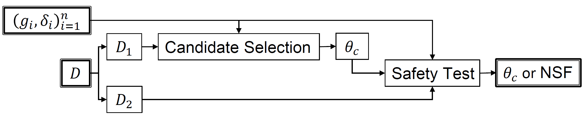 Figure 1 - Figure S15 (supplemental materials) P. S. Thomas, B. Castro da Silva, A. G. Barto, S. Giguere, Y. Brun, and E. Brunskill. Preventing undesirable behavior of intelligent machines. Science, 366:999–1004, 2019. Reprinted with permission from AAAS. A common misconception is that this algorithm is the Seldonian algorithm. There is no such thing, just as there is no one algorithm that is the reinforcement learning algorithm. This is one example of a Seldonian algorithm.
At a high level, Seldonian algorithms of this structure operate as follows. First, the available data \(D\) is partitioned into two sets, \(D_1\) and \(D_2\). After the publication of this figure in the original paper, we realized that it is not easy for people to remember which data set is \(D_1\) and which is \(D_2\). So, we have begun calling these the candidate data \(D_\text{cand}=D_1\) and the safety data \(D_\text{safety}=D_2\). $D_\text{cand}$ is provided as input to a component called candidate selection that selects a single solution that the algorithm plans to return. This solution is called the candidate solution \(\theta_c\). For now, you can imagine that candidate selection is your favorite off-the-shelf machine learning algorithm with no safety or fairness guarantees.
Next, the candidate solution is provided as input to a component called safety test (or sometimes the fairness test for algorithms designed specifically for fairness applications). The safety test mechanism uses the safety data \(D_\text{safety}=D_2\) to determine whether the algorithm is sufficiently confident that \(\theta_c\) would be safe to return. If the safety test is sufficiently confident that the candidate solution \(\theta_c\) is safe, then it returns \(\theta_c\). Otherwise, it returns No Solution Found (NSF). The safety test component is responsible for ensuring that the algorithm is Seldonian.
This algorithm structure should be natural, as it is what most data scientists would do if tasked with finding a machine learning model that is safe with high confidence. That is, they would train their model using some of the data (candidate selection) and would then use held-out data to verify that the model performs safely on unseen data (safety test). So, Seldonian algorithms essentially automate the exact process that a data scientist would follow.
This toolkit implements Seldonian algorithms with this general structure. In the following sections, we describe the safety test and candidate selection components in more detail. However, first we remind the reader that this algorithm structure is just one way that a Seldonian algorithm could be constructed. For example, the reinforcement learning algorithm presented in the Science paper performs the safety test before candidate selection.
Safety test
For simplicity, we begin by considering a simplified setting that limits the set of possible definitions of \(g_i\). Later in the "parse tree" section, we show how this simplified setting can be extended to allow for more complicated definitions of \(g_i\). For now, we assume:
- The data \(D\) consists of \(m\) independent and identically distributed (i.i.d.) data points. In the supervised learning setting, each data point is an input-label pair \((X_j,Y_j)\), while in the reinforcement learning setting, each data point corresponds to an entire episode of data. Furthermore, let \(m_c\) and \(m_s\) be the sizes of the candidate and safety data sets, respectively, so that \(m_c + m_s = m\). This assumption is not removed later.
- There is only a single behavioral constraint. That is, \(n=1\). We can therefore drop the \(i\) subscript and write \(\Pr(g(a(D))\leq 0)\geq 1-\delta\) rather than \(\Pr(g_i(a(D))\leq 0)\geq 1-\delta_i\). Later, we describe the simple extension to enable multiple constraints.
- The user specifies the desired definition of \(g\) by providing a function \(\hat g\) that uses data to construct unbiased estimates of \(g(\theta)\). That is, \(g(\theta)=\mathbf{E}[\hat g(\theta,D)]\), where here \(D\) could be any subset of the available data (it could be \(D\), \(D_c\), \(D_s\), or any other set of i.i.d. data points). This is the key limiting assumption that is removed in the "parse tree" section below. However, many definitions of \(g\) do satisfy this constraint.
The third assumption can be difficult to understand in this abstract form. To make it more concrete, consider an example: a regression problem where \(D=(X_j,Y_j)_{j=1}^m\), and where the goal is to minimize the mean squared error \(\operatorname{MSE}(\theta)=\mathbf{E}[(Y_j-\hat y(X_j,\theta))^2]\), where \(\hat y(X_j,\theta)\) is the regression model's prediction of \(Y_j\) based on the input \(X_j\) and using model parameters (weights) \(\theta\). Now, imagine that the user of the algorithm wants to add in the safety constraint that \(\operatorname{MSE}(\theta) \leq 2.0\), i.e., that the model is sufficiently accurate when applied to future points not seen during training. This constraint corresponds to \(g(\theta) = \operatorname{MSE}(\theta) - 2.0\), because \(\theta\) is considered safe if and only if \(g(\theta) \leq 0\). In this case, the user could provide the function \(\hat g\) that returns one unbiased estimate of \(g(\theta)\) from each data point \((X_j,Y_j)\). This function would simply return the squared residual for the \(j^\text{th}\) point minus 2.0: \(\hat g(\theta,(X_j,Y_j)) = (Y_i - \hat y(X_j,\theta))^2 -2.0 \). If \(\hat g\) is provided with more than one point, it can return one unbiased estimate of \(g(\theta)\) for each provided point.
With these assumptions, it is relatively easy to create the safety test mechanism. In the safety test, \(\hat g\) is calculated from the candidate solution \(\theta_c\) and the safety data \(D_\text{safety}=D_2\). The result is an array of unbiased estimates of \(g(\theta_c)\). Let \(Z_1,\dotsc,Z_{m_s}\) be these unbiased estimates of \(g(\theta)\). Recall that since these estimates are i.i.d. and unbiased, we know that for any \(j\), \(\mathbf{E}[Z_j] = g(\theta)\). Next, the safety test constructs a \(1-\delta\) confidence upper bound on the expected value of \(Z_j\) using standard statistical tools like Hoeffding's inequality or Student's \(t\)-test. If this \(1-\delta\) confidence upper bound is at most zero, then the algorithm can conclude with confidence at least \(1-\delta\) that \(\theta_c\) is safe, and so it is returned. If the \(1-\delta\) confidence upper bound is greater than zero, the algorithm cannot conclude with sufficient confidence that \(\theta_c\) is safe, and so it returns No Solution Found (NSF) instead.
In order to convert this English description of the safety test into a precise mathematical statement, we first review Student's \(t\)-test.
Student's \(t\)-test
Let \(Z_1,\dotsc,Z_m\) be \(m\) i.i.d. random variables and let \(\bar Z = \frac{1}{m}\sum_{i=1}^m Z_i\). If \(\bar Z\) is normally distributed, then for any \(\delta \in (0,1)\):
$$\Pr\left (\mathbf{E}[Z_1] \leq \bar Z + \frac{\hat \sigma}{\sqrt{m}}t_{1-\delta,m-1}\right ) \geq 1-\delta,$$
where \(\hat \sigma\) is the sample standard deviation including Bessel's correction:
$$\hat \sigma = \sqrt{\frac{1}{m-1}\sum_{i=1}^m{ \left( Z_i - \bar Z\right )^2}},$$
and where \(t_{1-\delta, \nu}\) is the \(100(1-\delta)\) percentile of the Student \(t\)-distribution with \(\nu\) degrees of freedom, i.e., tinv\((1-\delta,\nu)\) in Matlab.
To ground this abstract definition, consider an example. Imagine that we randomly selected \(m=30\) people from Earth (with replacement), and we measured their height in meters. Let these measurements be \(Z_1,\dotsc,Z_m\). These can be thought of as \(m\) i.i.d. samples of a random variable \(Z\) that corresponds to a randomly selected human's height. Student's \(t\)-test as described here would then provide a high-confidence upper bound on the average human height, \(\mathbf{E}[Z]\). However, it relies on the assumption that \(\frac{1}{m}\sum_{i=1}^m Z_i\) is normally distributed. This assumption is likely false, but it is reasonable due to the central limit theorem. If the average height measurement is \(\bar Z=1.76m\) and the sample standard deviation of the measured heights is \(\hat \sigma=0.07m\), then we can apply Student's \(t\)-test to obtain a \(1-\delta\) confidence upper bound on the true (unknown because we only measured the heights of 30 people) average human height. Using \(\delta=0.1\) we obtain a \(0.9\)-confidence upper bound on the average human height of
$$
\bar Z + \frac{\hat \sigma}{\sqrt{m}}t_{1-\delta,m-1} \approx 1.76m + \frac{0.07m}{\sqrt{30}}1.31 \approx 1.78m,
$$
where \(\approx\) is used when real numbers (like the value of \(t_{0.9,29}\)) are rounded. So, from this experiment, we could conclude with confidence \(0.9\) that the average human height is at most 1.78 meters.
Recall that in the safety test we apply Student's \(t\)-test to the outputs of \(\hat g(\theta_c, D_\text{safety})\) to obtain a \(1-\delta\)-confidence upper bound on \(g(\theta_c)\). Bringing together all the pieces, the safety test executes the following steps:
- Compute \(\hat g(\theta_c, D_\text{safety})\), which produces as output unbiased estimates \(Z_1,\dotsc,Z_{m_s}\). Note: In general, \(\hat g\) might output any number of unbiased estimates of \(g(\theta_c)\). In our example, \(\hat g\) returns one estimate per data point, so here we use \(m_s\) (the number of points in the safety set) to denote the number of unbiased estimates produced by \(\hat g\). Also, recall that for our grounding example, \(Z_j\) corresponds to the squared residuals on the \(j^\text{th}\) data point minus \(2.0\).
- Compute the sample mean \(\bar Z = \frac{1}{m_s}\sum_{j=1}^{m_s}Z_j\).
- Compute the sample standard deviation \(\hat \sigma = \sqrt{\frac{1}{m_s-1}\sum_{i=1}^{m_s} \left ( Z_i - \bar Z\right )^2}\).
-
Compute a \(1-\delta\) confidence upper bound \(U\) on \(g(\theta_c)\) using Student's \(t\)-test. That is, \(U = \bar Z + \frac{\hat \sigma}{\sqrt{m_s}}t_{1-\delta,m_s-1}\).
- If \(U \leq 0\), return \(\theta_c\), otherwise return No Solution Found (NSF).
One nice property of the safety test is that it operates properly regardless of how \(\theta_c\) is chosen. This means that in theory any off-the-shelf machine learning algorithm could be used for the candidate selection component. However, in practice this would not be very effective if the candidate selection mechanism often returns solutions that are not safe (the algorithm would often return NSF). In the next section, we discuss how the candidate selection mechanism can be designed to enable the algorithm to return NSF infrequently.
Candidate selection
As discussed at the end of the previous section, any off-the-shelf machine learning algorithm could be used for the candidate selection component. Currently the toolkit only supports parametric machine learning models (future versions may support non parametric models such as decision trees/random forests and support vector machines). Most off-the-shelf models will tend to be ineffective, however. There are two issues. First, standard machine learning algorithms may not consider safety at all, and if they frequently return unsafe solutions, the subsequent safety test will frequently return NSF. Second, even when standard machine learning algorithms do consider safety, they do not account for the details of the safety test that will be run. A more sophisticated candidate selection mechanism should consider the exact form of the subsequent safety test, and it should return candidate solutions that are likely to pass the safety test.
In this toolkit, we provide a candidate selection mechanism that searches for the candidate solution \(\theta_c\) that optimizes a typical primary objective function (e.g., minimize classification loss or maximize off-policy estimates of the expected return in the reinforcement learning setting) subject to the constraint that candidate selection predicts that the solution will pass the subsequent safety test. Candidate selection cannot actually compute whether or not the safety test will be passed because it does not have access to \(D_\text{safety}\). Using \(\hat f(\theta,D_\text{cand})\) to denote a primary objective function that should be maximized, we can then write an expression for the candidate solution:
$$
\theta_c \in \arg\max_{\theta \in \Theta}\hat f(\theta,D_\text{cand})\\\text{s.t. $\theta_c$ is predicted to pass the safety test}.
$$
This raises the question: how exactly should the safety test be predicted? This depends on the statistical tool used to compute the high-confidence upper bound on \(g(\theta_c)\). We use the following heuristic when using Student's \(t\)-test:
$$\theta_c \in \arg\max_{\theta \in \Theta}\hat f(\theta,D_\text{cand})\\\text{s.t. }\forall i \in \{1,2,\dotsc,n\},\quad \bar Z_i + 2\frac{\hat \sigma_i}{\sqrt{|D_\text{safety}|}}t_{1-\delta_i,|D_\text{safety}|-1}\leq 0,$$
where \(\bar Z_i\) and \(\hat \sigma_i\) are the sample mean and standard deviation of the unbiased estimate of the $i$th constraint computed from the candidate data, i.e., the sample mean and standard deviation of \(g_i(\theta,D_\text{cand})\). Notice that the only information about $D_\text{safety}$ that appears in this term is the size, $|D_\text{safety}|$. No actual safety data are used in this prediction, as that would constitute data leakage from the safety test to candidate selection.
We reiterate that this prediction of the safety test is a heuristic (one that we have found to be quite effective), not the result of a principled derivation. In particular, the constant \(2\) scaling the confidence interval from Student's \(t\)-test is chosen arbitrarily, and often other values work better in practice (in one case, we found that a factor of \(3\) was more effective). We expect that this is one aspect of Seldonian algorithms that could be improved.
The expression above describes the desired value of \(\theta_c\) as the solution to a constrained optimization problem. This raises the question: How should candidate selection compute or approximate the solution to this optimization problem? The Seldonian Toolkit allows the user to select an optimizer. As a starting point, it includes the CMA-ES algorithm using a boundary function to incorporate the constraint. This is the gradient-free black-box optimizer that was used in several papers presenting Seldonian algorithms. Though it can be effective for small problems, it tends to be too slow for larger problems. To overcome this limitation, we also include a gradient-based optimizer.
The gradient-based optimizer uses gradient descent with adaptive step-size schedules (Adam by default). However, notice that we cannot directly use gradient ascent (or descent), because the problem is constrained. This can be overcome using the KKT conditions (a generalization of Lagrange multipliers). We describe our approach below.
Optimization using the KKT conditions
The KKT theorem states that solutions to the constrained optimization problem:
$$\text{Optimize $f({\theta})$ subject to:}\\
h_i({\theta}){\leq}0, {\quad} i \in \{1,2,\dotsc,n\}$$
are the saddle points of the following Lagrangian function:
$${\mathcal{L(\mathbf{\theta,\lambda})}} = f(\mathbf{\theta}) + {\sum}_{i=1}^{n} {\lambda_i} h_i(\theta),$$
where $\lambda_i$ are constants called the Lagrange multipliers.
In our case, $f(\theta)$ is the primary objective function, and $h_i(\theta)$ is the upper bound on the $i$th constraint function: $$h_i({\theta}) = U(g_i(\mathbf{\theta})).$$
To find the saddle points of ${\mathcal{L(\theta,\lambda)}}$, we use gradient descent to obtain the global minimum over ${\theta}$ and simultaneous gradient ascent to obtain the global maximum over the multipliers, ${\lambda_i}$. To perform gradient descent, we need to be able to compute the gradients:
$$ \frac{\partial \mathcal{L}}{\partial \theta} = \frac{\partial f(\theta)}{\partial \theta} + {\sum}_{i=1}^{n} {\lambda_i} \frac{\partial \left( U(g_i(\theta)) \right)}{\partial \theta}\\
{\text{and}}\\
\frac{\partial \mathcal{L}}{\partial \lambda} = {\sum}_{i=1}^{n} {U(g_i(\theta))}.
$$
Sometimes these gradients are known, but in particular in the case of calculating $\frac{\partial \left( U(g_i(\theta)) \right)}{\partial \theta}$, where the constraint function (or the upper bound function) could take on a wide range of forms, we use automatic differentiation to compute the gradients. Once these gradients are calculated, we can perform the update rules of gradient descent (ascent). By default, we use the Adam optimizer to define the update rules.
Parse tree
In the safety test section above, we considered a simplified setting where the user could provide a function, $\hat{g}(\theta,D)$, that constructs an unbiased estimate of the constraint function $g(\theta)$. In reality, this is rarely practical and can be impossible when there do not exist unbiased estimators of $g(\theta)$. Furthermore, one of the core principles of the Seldonian framework is that the users who are determining what "unsafe" or "unfair" means for the system are often not machine learning practitioners or even programmers. They should therefore not be expected to define and provide code for a function $\hat{g}_i$ for each $i \in \{1,2,\dotsc,n\}$. While we could provide some hardcoded $\hat{g_i}$ functions as part of the Seldonian Toolkit, this would severely limit the definitions of undesirable behavior that the user could specify.
The parse tree provides a bridge between users and the algorithm that allows users to define behavioral constraints using simple mathematical statements. The parse tree replaces the function ${\hat {g}}$ with a (often binary) tree representing a mathematical expression. The internal nodes of the tree are mathematical operators like addition, division, and absolute value. The leaves of the tree are either constants or "base variables" $z_j(\theta)$. Examples of base variables include the false positive rate of a binary classifier, the false positive rate given that points correspond to males, the mean squared error of a regression model, and the expected discounted return of a reinforcement learning policy. Just like with $g(\theta)$, each base variable $z_j(\theta)$ comes with a function $\hat z_j$ such that $z_j(\theta) = \mathbf{E}[\hat z_j(\theta,D)]$.
Though the parse tree makes Seldonian algorithms more complicated, it makes it easier for users to define complex safety and fairness constraints. Instead of providing code for each $\hat g_j$ (which requires users to be able to program and to understand unbiased estimators), users of Seldonian algorithms with the parse tree functionality can simply type a mathematical expression. This expression is then automatically parsed to construct the parse tree. Common base variables like the (conditional) mean squared error, (conditional) false positive rates, and expected discounted return can be used without users having to provide any code. More advanced users can also create their own base variables either by providing a method for computing confidence intervals on the desired $z_j(\theta)$ from data $D$ or by providing an unbiased estimator for $z_j(\theta)$ and selecting a standard confidence interval like Student's $t$-test.
At the highest level of abstraction, base variables only need to provide a way for high-confidence upper and lower bounds on $z_j(\theta)$ to be computed from $D$. However, in almost all cases this is achieved using functions $\hat z_j(\theta,D)$ that produce unbiased estimates of $z_j(\theta)$. These functions, $\hat z_j$, are called measure functions in the Seldonian Toolkit. Again, we have provided these measure functions for the most common base variables.
To obtain a high-confidence upper bound on $g(\theta)$ (the root node of the parse tree), Seldonian algorithms first compute confidence intervals for all base variables of the tree (the toolkit automatically determines whether one- or two-sided confidence intervals are required for each base variable). The confidence intervals are then propagated through the tree back to the root using interval arithmetic rules. The upper bound on the root node is $U(\hat{g}(\theta))$, which is a high-confidence upper bound on the original constraint function, $g(\theta)$. This provides a modular framework allowing users to build a wide array of constraints that is much more flexible than forcing users to select from a list of preprogrammed definitions of $\hat{g}(\theta)$.
To make the idea of parse trees more concrete, let's consider the fairness constraint used in the GPA regression example studied by Thomas et al. (2019). The goal of the problem is to accurately predict the GPAs of students from their scores on nine entrance examinations, subject to a fairness constraint. The fairness constraint that Thomas et al. considered is that the model should not overpredict or underpredict on average for people of different genders. Concretely, the mean error for men and the mean error for women should not differ by more than 0.05. One way to write this constraint as a mathematical statement is:
$$g(\theta) = \operatorname{abs}((\text{Mean_Error} \,|\, [\text{Male}]) - (\text{Mean_Error} \,|\, [\text{Female}])) - 0.05,$$
where $\operatorname{abs}$ is the absolute value function and $\text{Mean_Error} \,|\, [\text{Male}]$ means "Mean squared error given male." Notice that if $g(\theta) \leq 0$ then $\operatorname{abs}((\text{Mean_Error} \,|\, [\text{Male}]) - (\text{Mean_Error} \,|\, [\text{Female}])) \leq 0.05$. The parse tree for this $g(\theta)$ can be visualized as:
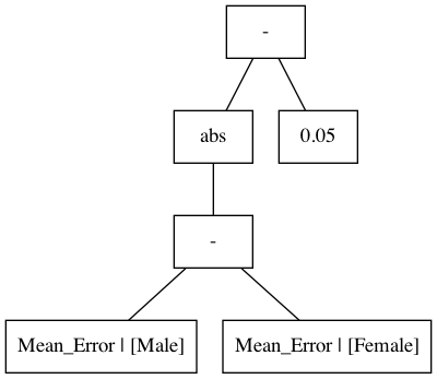 Figure 2 - Parse tree for the constraint: $g(\theta) = \operatorname{abs}((\text{Mean_Error} \,|\, [\text{Male}]) - (\text{Mean_Error} \,|\, [\text{Female}])) - 0.05$
In this example, the base variables are the two nodes at the bottom of the tree: $\text{Mean_Error} \,|\, [\text{Male}]$ and $\text{Mean_Error} \,|\, [\text{Female}]$. To calculate the high-confidence upper bound for this constraint, the high-confidence lower and upper bounds are first calculated on the two base variables using the $t$-test method described above. Then, these confidence bounds are propagated through the "-" node, representing the subtraction operator, just above those nodes. Next, the resulting confidence bound is propagated through the absolute value function. Finally, the confidence bound on the root node is calculated by propagating the resulting confidence bound and the bound from the constant node [0.05,0.05] through another subtraction operator, "-". The upper bound on $g$ is obtained from the upper bound on the root node. For example, let's say that in the safety test we calculated the confidence bounds on the base variables to be $[3.0,4.0]$ (male) and $[2.0,3.0]$ (female). The resulting confidence bounds on each node as they are propagated through the tree are shown in the following animation:
The resulting upper bound on the constraint is the upper bound on the root node, which is $1.95$ in this example. Since $1.95>0$, the safety test would reject the candidate solution in this case. Intuitively, this makes sense given that the intervals on the mean errors were $[3.0,4.0]$ (male) and $[2.0,3.0]$ (female), and the constraint is that the absolute difference of the mean errors must not differ by more than 0.05.