Seldonian ML
GitHub
Example: Seldonian reinforcement learning for safe diabetes treatment
The code and ideas in this tutorial began starting from a project conducted by Kimberley Faria and Chirag Sandeep Trasikar.
Contents
Background: Type 1 diabetes treatment as a reinforcement learning problem
Type 1 diabetes describes a condition where the body produces insufficient amounts of natural insulin. Insulin controls the delivery of glucose in the bloodstream to cells throughout the body. In doing so, it lowers the blood glucose concentration. People with untreated type 1 diabetes tend to have high blood glucose concentrations, a condition called hyperglycemia, which can have significant negative health consequences. One treatment for type 1 diabetes is the subcutaneous injection of synthetic insulin.
If too much synthetic insulin is injected, blood glucose levels can become dangerously low, a condition called hypoglycemia. Controlling hyperglycemia is important to prevent the long-term consequences of diabetes, and hypoglycemia is a common severe unintended consequence. The symptoms of hypoglycemia are often more acute and range from palpitations, sweating, and hunger, to altered mental status, confusion, coma, and even death.
In treating type 1 diabetes, it is critical to correctly estimate how much insulin a person should inject to mitigate hyperglycemia without inducing hypoglycemia. Synthetic insulin is usually delivered through "basal" injections, which regulate blood glucose between meals, and "bolus" injections, which are given just before mealtime to counteract the increase in blood glucose that results from eating a meal. Often, a bolus calculator is used to determine how much bolus insulin one should inject prior to eating a meal. This calculator is often personalized by a physician based on patient data. In this example, we show how to use the Seldonian Toolkit to create a reinforcement learning (RL) algorithm that personalizes the parameters of a bolus calculator to mitigate hyperglycemia, while ensuring with high confidence that dangerously low blood glucose levels are avoided.
The optimization of the parameters of a bolus calculator for Type 1 diabetes treatment can be framed as a RL problem, where finding the optimal policy, $\pi^{*}(s,a)$, is equivalent to optimizing the parameters of the bolus calculator for a single patient. We consider an episode to be a single day of patient data during treatment. For each episode, there is a single action, $a$, which is the selection of the parameters of the bolus calculator at the beginning of that day. The state, $s$, is a complete description of the person throughout the day, though the only part of the state that we observe is the patient's blood glucose levels. At three minute intervals throughout the day, the blood glucose levels are measured, and an instantaneous reward is assigned based on the difference between the measured blood glucose level and a target blood glucose level, typically determined by a physician. This reward function intuitively should penalize departures from healthy blood glucose concentrations, with worse penalties for hypoglycemia compared to hyperglycemia. At the end of the day, the mean of the instantaneous rewards is calculated and is considered to be the single reward for the episode.
Note: this example is a proof of concept, and the actual use of RL for automating type 1 diabetes treatment should be conducted by a team of medical researchers with proper safety measures and IRB approval. Individuals should not use this to modify their own treatments.
Formalizing the Seldonian RL problem
In this section, we formalize the RL problem and the safety constraint we will enforce using the Seldonian Toolkit. The RL policy $\pi(s,a)$ is parameterized by a bolus calculator, which determines the amount of insulin to inject before each meal. The particular parameterization we will use is:
$$
\begin{equation}
\text{injection} = \frac{\text{carbohydrate content of meal}}{CR} + \frac{\text{blood glucose} - \text{target blood glucose}}{CF},
\label{crcf_equation}
\end{equation}
$$
where the "carbohydrate content of meal" is an estimate of the size of the meal to be eaten (measured in grams of carbohydrates), "blood glucose" is an estimate of the person’s current blood glucose concentration (measured from a blood sample and using milligrams per deciliter of blood, i.e., mg/dL), "target blood glucose" is the desired blood glucose concentration (also measured using mg/dL, typically specified by a physician), and $CR$ and $CF$ are two real-valued parameters that, for each person, must be tuned to make the treatment policy effective. $CR$ is the carbohydrate-to-insulin ratio, and is measured in grams of carbohydrates per insulin unit, while $CF$ is called the correction factor or insulin sensitivity, and is measured in mg/dL per insulin unit.
In a realistic treatment scenario, a physician might propose an initial range of $CR,CF$ values and may want to know what is the best sub-range in $(CR,CF)$ space for a particular patient. This is equivalent to finding an optimal distribution over policies $d^{*}(\pi(s,a))$, rather than a single optimal policy.
Using a standard RL algorithm, one could obtain an optimal policy distribution by maximizing the expected return of a reward function. However, there would be no guarantee that the optimal policy distribution was actually safe when deployed for that patient. A reasonable concern is that even though the chosen reward function might disincentivize hypoglycemia, there is still a chance of it occurring, and one would not know what that chance is. What we desire is a high level of confidence that the deployed bolus controller (with $CR,CF$ values taken from the obtained distribution over policies) will reduce the prevalence of hypoglycemia compared to the bolus controller that uses the larger range of initially-proposed $CR,CF$ values. To achieve this, we consider two reward functions: i) a primary reward function that disincentivizes both hyperglycemia and hypoglycemia, and ii) an auxiliary reward function that only disincentivizes hypoglycemia, which we will use in the safety constraint.
We select an instantaneous primary reward function that approximates the one proposed by Bastani (2014), who studied the non-Seldonian version of this problem in detail. We define our instantaneous primary reward function $r_0(t)$ as:
$$
\begin{equation}
r_0(t) =
\begin{cases}
-1.5*10^{-8}*|g_t - 108 | & g_t < 108 \\
-1.6*10^{-4}*(g_t - 108 )^2 & g_t \geq 108 \\
\end{cases}
\label{primary_reward}
\end{equation}
$$
where $g_t$ is the blood glucose concentration at time $t$ in mg/dL and 108 is the target blood glucose value. The instantaneous reward function from Equation \ref{primary_reward} is shown in Figure 1.
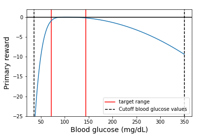 Figure 1: The instantaneous primary reward function (blue). All rewards are non-positive, with the best reward of 0 occurring when blood glucose concentration is the target value of 108 mg/dL. If the blood glucose concentration goes below 36 mg/dL or above 350 mg/dL, we stop the episode, as values outside of this range are unphysical.
The primary reward $r_0$ that gets assigned to an episode (a single day) is the mean of the instantaneous primary rewards throughout the day, i.e., $r_0 = \frac{1}{T}\sum_{t=0}^{T-1}{r_0(t)}$, where $T$ is the total number of times at which the blood glucose is measured in a day. If the blood glucose concentration goes beyond the physical range ($<36$ or $>350$ mg/dL), then we stop the episode and assign the minimum possible reward (the reward when $g_t=36$ mg/dL) for that timestep and all subsequent timesteps for the remainder of the episode.
The goal of the RL problem in the absence of constraints is to find a distribution over policies that optimizes the primary expected return $J_{0,d(\pi)} = \frac{1}{m} \sum_{i=0}^{m-1}{r_{0,i}}$, where $m$ is the total number of episodes (days) in the dataset, and $r_{0,i}$ is the primary reward for the $i$th episode. The Seldonian RL optimization problem seeks to simultaneously optimize $J_{0,d(\pi)}$ and enforce the safety constraint(s). Here we have a single safety constraint, which is that the incidence of hypoglycemia of the obtained distribution over policies must be lower than that of the initially-proposed distributon over policies. To quantify the incidence of hypoglycemica, we define an auxiliary instantaneous reward function, $r_1(t)$:
$$
\begin{equation}
r_1(t) =
\begin{cases}
-1.5*10^{-8}*|g_t - 108 | & g_t < 108 \\
0 & g_t \geq 108 \\
\end{cases}
\label{aux_reward}
\end{equation}
$$
This is identical to the primary instantaneous reward function (Equation \ref{primary_reward}) when $g_t < 108 $. The auxiliary reward for a single day is $r_1 = \frac{1}{T}\sum_{t=0}^{T-1}{r_1(t)}$, where $T$ is the total number of times at which the blood glucose is measured in a day. The auxiliary expected return is $J_{1,d(\pi)} = \frac{1}{m} \sum_{i=0}^{m-1}{r_{1,i}}$, where $m$ is the total number of episodes (days) in the dataset, and $r_{1,i}$ is the auxiliary reward for the $i$th episode. The safety constraint we described above can be written formally:
$$
\begin{equation}
J_{1,d_{\text{new}}(\pi)} \geq J_{1,d_b(\pi)},
\label{constraint}
\end{equation}
$$
where $d_{\text{new}}(\pi)$ is the new policy distribution and $d_b(\pi)$ is the behavior policy distribution.
Implementation details
To simulate a patient's treatment data with a bolus calculator, we used simglucose, an open source Python approximation of the closed-source FDA-approved UVa/Padova Simulator (2008 version). The default controller in simglucose is a basal-only controller. Because we were interested in studying the bolus-only problem, we forked the simglucose github repository and added a bolus-only controller. We also created a custom RL gym environment in our simglucose fork so that we could use the primary and auxiliary reward functions (Equations \ref{primary_reward} and \ref{aux_reward}) defined in the previous section. Our simglucose fork can be found here.
Simglucose provides thirty virtual patients with unique metabolic parameters spanning the type 1 diabetes population. However, many patients' blood glucose concentrations reach unphysical values within a few hours for all reasonable pairs of $CR,CF$, such that policy improvement algorithms will be ineffective. For this example, we chose adult#008, because their blood glucose levels were less volatile, at least for some combinations of $CR,CF$. A single simglucose simulation samples the blood glucose concentration of the patient once every three minutes over the course of a single day. The meals of each day are structured as follows: there are three possible larger meals and a possible snack after each meal. The probability of each large meal occurring is 0.95, and the probability of each snack occurring is 0.3. Meal times and amounts are sampled from truncated normal distributions (for details, see the simglucose source code).
We ran simglucose simulations for this patient over a large grid of $CR$ and $CF$ values: $CR \in [5,45]$ with a spacing of 5, $CF \in [1,28]$ with a spacing of 3. At each $CR,CF$ pair, we generated 20 episodes (days) of data. In Figure 2, we plot the primary and auxiliary rewards (the mean over each day of the instantaneous rewards from Equations \ref{primary_reward} and \ref{aux_reward}) over this range of CR and CF values.
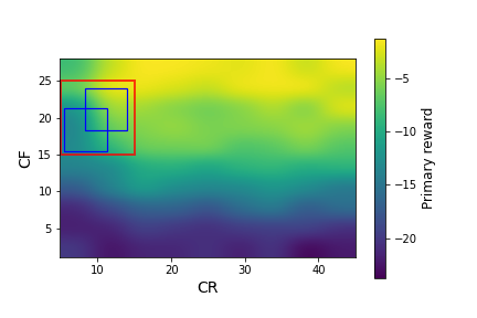
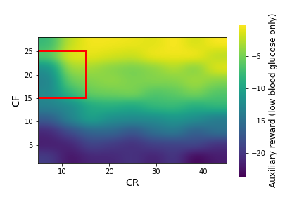 Figure 2: The primary rewards (left) and auxiliary rewards (right) as a function of $CR$ and $CF$ for the adult#008 simglucose patient, after smoothing with a Gaussian kernel. The red square indicates the box that we use as the initial policy distribution. The blue squares in the left plot indicate possible policy distributions.
Figure 2 shows large variations in the primary and auxiliary rewards, with a strong dependence on $CF$ and a weaker dependence on $CR$. A physician would not have access to these data before beginning to treat a patient. Instead, they would decide initial values of $CR$ and $CF$ based on their expertise and patient-specific information they have collected. In this example, we consider the case where the physician specifies the red box in Figure 2 as $d_b(\pi)$, the behavior policy distribution. This corresponds to:
$$
\begin{equation}
CR \in (5,15)\\ CF \in (15,25)
\label{behavior_policy_box}
\end{equation}
$$
Below we show two simulated episodes with $CR,CF$ values that fall within the red box in Figure 2.
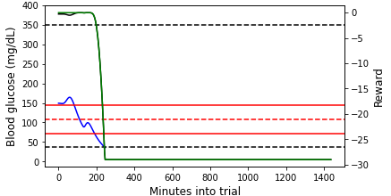
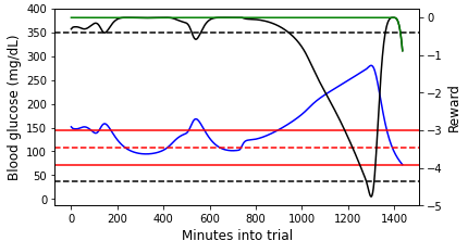
 Figure 3: (Left) An example episode that we terminated due to the patient reaching unphysical blood glucose (bg) levels partway into the day ($CR=5$, $CF=25$). (Right) An episode that lasts for the entire day ($CR=15$, $CF=22$). In both plots, the blood glucose values are shown on the primary y-axis, and the (instantaneous) reward values are shown on the secondary y-axis. Note that the Python simulator we used is an imperfect approximation of the FDA approved simulator. For this reason, the simulation results may not be precisely realistic.
For the episode shown in the left plot of Figure 3, the blood glucose concentration quickly plummets and does not recover before hitting the unphysically low blood glucose level. The primary and auxiliary instantaneous rewards also decline rapidly, hitting the minimum reward floor once the unphysical blood glucose level is reached. At the beginning of the episode shown in the right plot of Figure 3, the blood glucose concentration stays within or just above the target range. During this time, the primary reward is close to maximum and the auxiliary reward is 0 because the blood glucose value is not lower than the target value (c.f., Equations \ref{primary_reward} and \ref{aux_reward}). As the blood glucose rises outside of the target range, the primary instantaneous reward declines. At the very end of the episode, the blood glucose drops below the target value (though still in the target range), and both the primary and auxiliary instantaneous rewards (which are now equal at this point) drop.
Our goal in this example is to use the Seldonian toolkit to obtain a policy distribution $d_{\text{new}}(\pi)$, that has higher primary expected return $J_{0,d_{\text{new}}(\pi)}$ than that of the behavior policy distribution $J_{0,d_b(\pi)}$ and that satisfies the safety constraint (Equation \ref{constraint}). In order to evaluate the performance and safety of the new policy distribution against the behavior policy distribution, we must first calculate those quantities for the behavior policy distribution. To do this, we used simglucose to simulate five thousand episodes (days) of patient data (blood glucose concentration measurements) under the behavior policy distribution. For a given episode, the action is the selection of $CR$ and $CF$, which are sampled from uniform random distributions between the endpoints described by the behavior policy distribution box (Equation \ref{behavior_policy_box}). We obtained a primary expected return of $J_{0,d_b(\pi)} \simeq -6.1$ and an auxiliary expected return of $J_{1,d_b(\pi)} \simeq -5.4$. We can now write our safety constraint quantitatively as:
$$
\begin{equation}
J_{1,d_{\text{new}}(\pi)} \geq -5.4.
\label{constraint_withnumbers}
\end{equation}
$$
An important implementation detail is deciding the size/shape of new policy distributions, i.e., smaller sub-boxes within the initial policy distribution box. We first attempted to parameterize new policy distributions simply as the edges of a box, with no constraints on the shape or area of the box other than that it had to fall entirely within the bounds initial policy distribution box. This approach led to overfitting, where the Seldonian algorithm pushed the size of the box to be so small that it only contained a few episodes. Even mitigating this with regularization strategies penalizing the inverse area of the box did not fully resolve the overfitting issue.
Ultimately, we decided to fix the new policy distributions to be squares with one third of the area of the behavior policy distribution square. This simplifies our parameter space to two dimensions, i.e., the center of the box in $(CR,CF)$. The blue squares in the left plot of Figure 2 show two example policy distributions. The bounds of the square are real numbers, so even with this simplification there is a vast parameter space to explore. Because the parameter space is bounded, and our KKT optimization procedure works best for unbounded variables, we introduced a mapping between the centers of the policy distribution box $(CR_{\text{cen}}$, $CF_{\text{cen}})$ and the unbounded parameters $\theta_1 \in (-\infty,+\infty)$, $\theta_2 \in (-\infty,+\infty)$ that we use in the optimization procedure.
$$
\begin{equation}
CR_{\text{cen}} = \sigma(\theta_1)*CR_{\text{size}} + CR_{\text{min}} \\
CF_{\text{cen}} = \sigma(\theta_2)*CF_{\text{size}} + CF_{\text{min}},
\label{theta2crcf}
\end{equation}
$$
where $\sigma(x)$ is the sigmoid function, $CR_{\text{size}}$ and $CF_{\text{size}}$ are the sizes of the new policy distribution box in $CR$ and $CF$ space, respectively, and $CR_{\text{min}}$ and $CF_{\text{min}}$ are the minimum possible values for $CR_{\text{cen}}$ and $CF_{\text{cen}}$, respectively, that keep the square inside of the original policy distribution box. Because we fixed the new policy distribution boxes to have 1/3 of the area of the original policy distribution box, the sizes of the new policy distribution boxes in $CR$ and $CF$ space are $\frac{1}{\sqrt{3}}$ times the original sizes, i.e., $CR_{\text{size}} = CF_{\text{size}} = \frac{10}{\sqrt{3}}$. This constraint also requires that $CR_{\text{min}} = 5 + \frac{10}{2\sqrt{3}}$ and $CF_{\text{min}} = 15 + \frac{10}{2\sqrt{3}}$.
A final implementation detail is the method with which we estimated the expected return of new policies. As with any high-risk RL application, off-policy evaluation is preferred for estimating the performance of proposed policies because many of these policies may be harmful or even fatal. In this example, we use importance sampling with unequal support (US) as the off-policy estimator, introduced by Thomas and Brunskill (2017). This method is fast to compute and has lower variance than other common importance sampling estimators for this particular setting.
Running a Seldonian Experiment
The first step in running a Seldonian Experiment is generating a specification ("spec") object. For RL problems, the dataset component of the spec object must consist of episodes generated by the behavior policy (or behavior policy distribution, in this case). We generated 2500 of such episodes using the following script called generate_data.py.
# generate_data.py
import time
import autograd.numpy as np
import concurrent.futures
from tqdm import tqdm

import gym
from gym.envs.registration import register
from simglucose.controller.bolus_only_controller import BolusController

from seldonian.dataset import Episode
from seldonian.utils.io_utils import save_pickle

# Globals
ID = "simglucose-adult8-v0"
patient_name = "adult#008"
S_0 = 0 # initial state
# "Physician" specified bounds
CR_min = 5.0
CR_max = 15.0
CF_min = 15.0
CF_max = 25.0
MAX_TIMESTEPS = 480 # 480 minutes is a day at 3 minutes per timestep
target_BG = 108 # mg/dL
low_cutoff_BG = 36
high_cutoff_BG = 350
min_primary_reward = -1.5e-8*np.abs(low_cutoff_BG-target_BG)**5
min_secondary_reward = min_primary_reward

def run_simulation(env):
    "Run a single simglucose simulation given a gym env"
    observation, reward, alt_reward,done, info = env.reset()
    primary_return = reward
    alt_return = alt_reward

    cr = np.random.uniform(CR_min,CR_max)
    cf = np.random.uniform(CF_min,CF_max)
    controller = BolusController(cr=cr, cf=cf, target=target_BG)

    t = 0
    start_time = time.time()
    primary_rewards = min_primary_reward*np.ones(MAX_TIMESTEPS)
    alt_rewards = min_secondary_reward*np.ones(MAX_TIMESTEPS)
    while not done:
        action = controller.policy(
            observation,
            reward,
            done,
            patient_name=patient_name,
            meal=info['meal'])
        observation, primary_reward, alt_reward, done, info = env.step(action)
        primary_rewards[t] = primary_reward
        alt_rewards[t] = alt_reward
        t += 1
        if t == MAX_TIMESTEPS:
            done=True
        if done:
            print(f"Episode finished after {t} (sample) timesteps, Simulation run time = {time.time() - start_time} secs.")
            break
    primary_return = np.mean(primary_rewards)
    alt_return = np.mean(alt_rewards)
    return t, cr, cf, primary_return, alt_return

def run_simglucose_trial(env):
    "Wrapper to call run_simulation(). Return an Episode() object"
    t, cr_action, cf_action, reward, alt_reward = run_simulation(env)

    observations = [S_0]
    actions = [(cr_action,cf_action)]
    prob_actions = [0.]
    rewards = [reward]
    alt_rewards = np.array([[alt_reward,],])
    # That's the end of the episode, so return the history
    return Episode(observations, actions, rewards, prob_actions, alt_rewards=alt_rewards)


def deregister_and_register_env(ID,patient_name,custom_scenario=None,target=108):
    deregister_env(ID)
    register_env(
        ID=ID,
        patient_name=patient_name,
        custom_scenario=custom_scenario,
        target=target
    )
    return

def register_env(ID,patient_name,custom_scenario=None,target=108):
    register(
        id=ID,
        entry_point='simglucose.envs:CustomT1DSimEnv',
        kwargs={
            'patient_name': patient_name,
            'custom_scenario': custom_scenario,
            'target': target
        }
    )
    return


def deregister_env(ID):
    env_dict = gym.envs.registration.registry.env_specs.copy()

    for env in env_dict:
        if ID in env:
            del gym.envs.registration.registry.env_specs[env]


def func_to_parallelize(num_episodes):
    """ Function that is run in parallel. Runs num_episodes episodes
    on a single core
    """
    deregister_and_register_env(ID,patient_name,target=target_BG)
    env = gym.make(ID)

    episodes = []
    secondary_returns = []

    for i in range(num_episodes):
        ep = run_simglucose_trial(env)
        secondary_returns.append(ep.alt_rewards[0][0])
        episodes.append(ep)

    return episodes

if __name__ == '__main__':
    NUM_EPISODES = 2500
    num_cpus = 7
    chunk_size = NUM_EPISODES // num_cpus
    chunk_sizes = []
    for i in range(0,NUM_EPISODES,chunk_size):
        if (i+chunk_size) > NUM_EPISODES:
            chunk_sizes.append(NUM_EPISODES-i)
        else:
            chunk_sizes.append(chunk_size)
    with concurrent.futures.ProcessPoolExecutor(max_workers=num_cpus) as executor:

        # Map the parallel function to chunks of episodes
        results = tqdm(executor.map(func_to_parallelize, chunk_sizes),total=len(chunk_sizes))

        # Concatenate the results from all processes into a single list
        episodes = [item for sublist in results for item in sublist]
    # Print the squared list
    os.makedirs('./data',exist_ok=True)
    EPISODES_FILE = f'./data/simglucose_adult#008_customreward_{NUM_EPISODES}episodes.pkl'
    save_pickle(EPISODES_FILE, episodes, verbose=True)
Running this Python script will produce a directory called data/, and inside it a file called simglucose_adult#008_customreward_2500episodes.pkl. This file contains a list of Episode() objects, which we will use in the next script to create the specification object.
The specfication object contains all of the information we will need to run the Seldonian algorithm, including the dataset, model (policy parameterization), optimization method, hyperparameters, and our safety constraint. Below is a script which we named create_spec.py that creates the specification object. Note that due to the nature of our policy parameterization, the gradient-based KKT optimization method will be ineffective. This is because small changes to the current range of CR and CF values may not change which episodes fall inside and outside of the current box, resulting in identical off-policy estimates, and the gradient of the OPE estimates with respect to the policy parameters will typically be either zero or undefined. Our parameter space is small, so we can use black box optimization with a barrier function instead of KKT. We will use the CMA-ES optimizer with an initial standard deviation of 5 for both $\theta_1$ and $\theta_2$.
Note the constraint string: 'J_pi_new_US_[1] >= -5.4'. Here, J_pi_new_US refers to the performance of the new policy evaluated using importance sampling with unequal support (US). The _[1] suffix references the 1st auxiliary reward. If this suffix is omitted, the performance of the primary reward is used by default. In the generate_data.py script above, we included in our episode objects a single auxiliary reward called alt_reward, and the toolkit _[1] suffix in the constraint instructs the toolkit to use this reward when evaluating the constraint. We created a new RL policy class for this problem called SigmoidPolicyFixedArea, which implements the transformation between $\theta$ and $CR,CF$, defined in Equation \ref{theta2crcf}. The source code for this policy can be found in this module.
# create_spec.py
import autograd.numpy as np
from seldonian.RL.Agents.Policies.SimglucosePolicyFixedArea import SigmoidPolicyFixedArea
from seldonian.spec import RLSpec
from seldonian.models import objectives
from seldonian.RL.RL_model import RL_model
from seldonian.parse_tree.parse_tree import make_parse_trees_from_constraints
from seldonian.dataset import RLDataSet,RLMetaData
from seldonian.utils.io_utils import load_pickle,save_pickle

# Physician specifies the bounding box in CR/CF space of possible values
# Our policy can never go outside of this box
CR_min = 5.0
CR_max = 15.0
CF_min = 15.0
CF_max = 25.0

def initial_solution_fn(x):
    # Draw random numbers for (theta1,theta2) to initialize the parameter search
    return np.random.uniform(-5,5,size=2)

def main():
    np.random.seed(42)

    NUM_EPISODES = 2500
    sigma0 = 5
    episodes_file = f'./data/simglucose_adult#008_customreward_{NUM_EPISODES}episodes.pkl'

    episodes = load_pickle(episodes_file)
    meta = RLMetaData(all_col_names=["episode_index", "O", "A", "R", "pi_b","R_1"])
    dataset = RLDataSet(episodes=episodes,meta=meta)
    frac_data_in_safety = 0.5

    # behavioral constraints
    constraint_strs = ['J_pi_new_US_[1] >= -5.4']
    deltas=[0.05]
    parse_trees = make_parse_trees_from_constraints(
        constraint_strs,
        deltas,
        regime="reinforcement_learning",
        sub_regime="all",
        columns=[],
        delta_weight_method="equal"
    )

    # Initialize policy and model
    policy = SigmoidPolicyFixedArea(
        bb_crmin=CR_min,
        bb_crmax=CR_max,
        bb_cfmin=CF_min,
        bb_cfmax=CF_max,
        cr_shrink_factor=np.sqrt(3),
        cf_shrink_factor=np.sqrt(3)
    )

    env_kwargs={'gamma':1.0} # gamma doesn't matter because our episode is only 1 timestep long
    model = RL_model(policy=policy, env_kwargs=env_kwargs)

    verbose=True
    spec = RLSpec(
        dataset=dataset,
        model=model,
        parse_trees=parse_trees,
        frac_data_in_safety=frac_data_in_safety,
        primary_objective=objectives.US_estimate,
        initial_solution_fn=initial_solution_fn,
        base_node_bound_method_dict={},
        use_builtin_primary_gradient_fn=False,
        optimization_technique="barrier_function",
        optimizer="CMA-ES",
        optimization_hyperparams={
            "sigma0": sigma0,
            "verbose": verbose
        },
        batch_size_safety=None,
        verbose=verbose
    )
    os.makedirs("./specfiles")
    spec_savename = f"specfiles/simglucose_adult#008_customreward_{NUM_EPISODES}episodes_sigma{sigma0}_fixedarea_spec.pkl"
    save_pickle(spec_savename,spec,verbose=True)

if __name__ == '__main__':
    main()
Running this script will create a directory called specfiles/ and inside of it a pickle file called simglucose_adult#008_customreward_2500episodes_sigma5_fixedarea_spec.pkl. We now have everything we need to run the Seldonian experiment.
The script below, run_experiment.py, runs an experiment with 100 trials over 10 log-spaced data fractions between $0.001$ and $1.0$, where a data fraction of $1.0$ corresponds to $m=2500$ episodes. Including the line near the top: os.environ["OMP_NUM_THREADS"] = "1" will vastly speed up parallel calculations for multi-core machines. For this problem, we created a new RL environment in the toolkit called SimglucoseCustomEnv (see: this module) and a new agent called SimglucoseFixedAreaAgent (see: this module). We define functions near the top of the file called create_env_func() and create_agent_func(), which create new environments and agents, respectively. These are used within the function generate_episodes_and_calc_J() to generate new episodes in order to evaluate the ground truth peformance and safety of new policies.
Another important parameter is n_episodes_for_eval=2000, which is the number of episodes we generate when evaluating each trial solution in generate_episodes_and_calc_J(). We set n_workers_for_episode_generation=46 and n_workers=1. The former is how many cores we use to generate both the trial episodes and the new episodes for evaluation, and the latter is how many cores we use to parallelize over trials. Our choice to parallelize over episode generation is due to the fact that the computational bottleneck is in generating episodes rather than running the Seldonian algorithm in each trial. For more details on how to efficiently parallelize toolkit code, see Tutorial M: Efficient parallelization with the toolkit.
We created a baseline for this experiment called RLDiabetesUSAgentBaseline, which performs an identical optimization as the Seldonian algorithm, except it does not consider the constraint and it does not have a safety test. That is, it just performs importance sampling with unequal support to optimize the expected return of the new policy. The source code for this baseline can be found in this module.
# run_experiment.py
from functools import partial
import os
os.environ["OMP_NUM_THREADS"] = "1"
import autograd.numpy as np   # Thinly-wrapped version of Numpy
from concurrent.futures import ProcessPoolExecutor
import multiprocessing as mp
from tqdm import tqdm

from seldonian.utils.io_utils import load_pickle
from seldonian.utils.stats_utils import weighted_sum_gamma
from seldonian.RL.RL_runner import run_episode,run_episodes_par
from seldonian.RL.environments.simglucose_custom import SimglucoseCustomEnv
from seldonian.RL.Agents.simglucose_custom_fixedarea_random_agent import SimglucoseFixedAreaAgent

from experiments.baselines.diabetes_US_baseline import RLDiabetesUSAgentBaseline
from experiments.generate_plots import RLPlotGenerator

CR_min = 5.0
CR_max = 15.0
CF_min = 15.0
CF_max = 25.0

def create_env_func():
    return SimglucoseCustomEnv(CR_min,CR_max,CF_min,CF_max)

def create_agent_func(new_params,cr_shrink_factor=1,cf_shrink_factor=1):
    agent = SimglucoseFixedAreaAgent(
        CR_min,
        CR_max,
        CF_min,
        CF_max,
        cr_shrink_factor=cr_shrink_factor,
        cf_shrink_factor=cf_shrink_factor
    )
    agent.set_new_params(new_params)
    return agent

def generate_episodes_and_calc_J(**kwargs):
    """ Calculate the expected discounted return
    by generating episodes

    :return: episodes, J, where episodes is the list
        of generated ground truth episodes and J is
        the expected discounted return
    :rtype: (List(Episode),float)
    """
    # Get trained model weights from running the Seldonian algo
    model = kwargs['model']
    num_episodes = kwargs['n_episodes_for_eval']
    hyperparameter_and_setting_dict = kwargs['hyperparameter_and_setting_dict']
    n_workers_for_episode_generation = hyperparameter_and_setting_dict['n_workers_for_episode_generation']

    new_params = model.policy.get_params()
    env_func_par = create_env_func
    agent_func_par = partial(
        create_agent_func,
        new_params=new_params,
        cr_shrink_factor=np.sqrt(3),
        cf_shrink_factor=np.sqrt(3)
    )

    episodes = []
    if n_workers_for_episode_generation > 1:
        chunk_size = num_episodes // n_workers_for_episode_generation
        chunk_sizes = []
        for i in range(0,num_episodes,chunk_size):
            if (i+chunk_size) > num_episodes:
                chunk_sizes.append(num_episodes-i)
            else:
                chunk_sizes.append(chunk_size)

        create_env_func_list = (env_func_par for _ in range(len(chunk_sizes)))
        create_agent_func_list = (agent_func_par for _ in range(len(chunk_sizes)))

        with ProcessPoolExecutor(
            max_workers=n_workers_for_episode_generation, mp_context=mp.get_context("fork")
        ) as ex:
            results = tqdm(
                ex.map(
                    run_episodes_par,
                    create_agent_func_list,
                    create_env_func_list,
                    chunk_sizes
                ),
                total=len(chunk_sizes)
            )
            for ep_list in results:
                episodes.extend(ep_list)
    else:
        env = create_env_func()
        agent = create_agent_func(new_params)
        for i in range(num_episodes):
            episodes.append(run_episode(agent,env))


    # Calculate J, the discounted sum of rewards
    returns = np.array([weighted_sum_gamma(ep.rewards,gamma=1.0) for ep in episodes])
    J = np.mean(returns)
    return episodes,J


def initial_solution_fn(x):
    return np.random.uniform(-5,5,size=2) # in theta space, not CR/CF space

if __name__ == "__main__":
    # Parameter setup
    np.random.seed(99)
    run_experiments = False
    make_plots = True
    save_plot = True
    include_legend= True
    model_label_dict = {
        "qsa": "Seldonian model"
    }
    NUM_EPISODES = 2500 # For making trial datasets and for looking up specfile
    n_episodes_for_eval = 2000
    sigma0=5
    performance_metric = 'J(pi_new)'
    n_trials = 100
    data_fracs = np.logspace(-3,0,10)
    n_workers_for_episode_generation = 46
    n_workers = 1
    verbose=True
    results_dir = f'results/simglucose_adult#008_customreward_{NUM_EPISODES}episodes_sigma{sigma0}_fixedarea_{n_episodes_for_eval}evaluation_{n_trials}trials'
    os.makedirs(results_dir,exist_ok=True)
    plot_savename = os.path.join(results_dir,f'simglucose_adult#008_customreward_fixedarea_{n_trials}trials.png')
    # Load spec
    specfile = f'./specfiles/simglucose_adult#008_customreward_{NUM_EPISODES}episodes_sigma{sigma0}_fixedarea_spec.pkl'
    spec = load_pickle(specfile)

    perf_eval_fn = generate_episodes_and_calc_J
    perf_eval_kwargs = {
        'n_episodes_for_eval':n_episodes_for_eval,
        'env_kwargs':spec.model.env_kwargs,
    }
    initial_solution = np.random.uniform(-10,10,size=2) # theta values
    # The setup for generating behavior data for the experiment trials.
    hyperparameter_and_setting_dict = {}
    hyperparameter_and_setting_dict["create_env_func"] = create_env_func
    hyperparameter_and_setting_dict["create_agent_func"] = partial(
        create_agent_func,
        new_params=initial_solution,
        cr_shrink_factor=1,
        cf_shrink_factor=1
    )
    hyperparameter_and_setting_dict["num_episodes"] = NUM_EPISODES
    hyperparameter_and_setting_dict["n_workers_for_episode_generation"] = n_workers_for_episode_generation
    hyperparameter_and_setting_dict["num_trials"] = 1 # Leave as 1 - it is not the same "trial" as experiment trial.
    hyperparameter_and_setting_dict["vis"] = False

    plot_generator = RLPlotGenerator(
        spec=spec,
        n_trials=n_trials,
        data_fracs=data_fracs,
        n_workers=n_workers,
        datagen_method='generate_episodes',
        hyperparameter_and_setting_dict=hyperparameter_and_setting_dict,
        perf_eval_fn=perf_eval_fn,
        perf_eval_kwargs=perf_eval_kwargs,
        results_dir=results_dir,
        )

    if run_experiments:
        env_kwargs = {'gamma':1.0}
        baseline_model = RLDiabetesUSAgentBaseline(initial_solution,env_kwargs)
        plot_generator.run_baseline_experiment(baseline_model=baseline_model,verbose=verbose)

        plot_generator.run_seldonian_experiment(verbose=verbose)

    if make_plots:
        plot_generator.make_plots(fontsize=12,legend_fontsize=8,
            performance_label=performance_metric,
            include_legend=include_legend,
            model_label_dict=model_label_dict,
            save_format="png",
            savename=plot_savename if save_plot else None)
Below we show the three experiment plots resulting from running the above script.
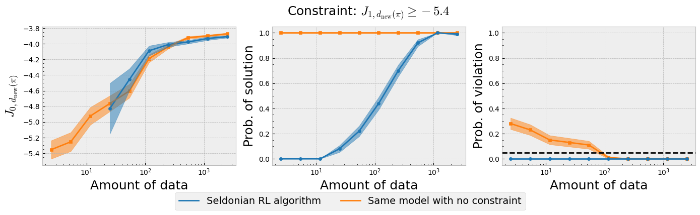 Figure 4: The three plots of the Seldonian experiment obtained using the Seldonian RL algorithm on the type 1 diabetes treament problem. The Seldonian RL algorithm (blue) is plotted alongside the baseline model (orange) that uses the same model but does not train it with the safety constraint. (Left) Performance, (middle) probability of solution, and (right) probability of violating the constraint for 100 trials as a function of the number of episodes (days) used as input to the Seldonian algorithm. The black dashed line in the right plot indicates $\delta=0.05$, i.e., the maximum allowable probability that the Seldonian algorithm violates the constraint. The performance $J_{0,d_{\text{new}}(\pi)}$ is the expected return of the primary reward of the new policy distribution obtained in each trial. The probability of solution represents the fraction of trials that passed the safety test in each trial. The probability of violating the constraint represents the fraction of trials that passed the safety test but then violated the safety constraint on ground truth data.
Figure 4 shows that the Seldonian RL algorithm was successful at achieving the goal we set in this example, which was to create an algorithm to find policy distributions (new sub-boxes in $CR,CF$ space) that improve the primary expected return (less incidence of both hyper and hypoglycemia) over the behavior policy distribution (initially proposed $CR,CF$ box), while ensuring with high confidence that hypoglycemic episodes were less prevalent. Recall that the primary expected return of the behavior policy distribution was $J_{0,d_b(\pi)}\simeq - 6.1$, which is exceeded by the Seldonian algorithm with less than 50 days of data (Figure 4; left plot). The Seldonian algorithm's primary expected return matches that of the baseline, indicating that satisfying the safety constraint does not require any trade-off in the primary return. This is not surprising given that the two reward functions are well-aligned, but it is still a good indication that the Seldonian algorithm is not doing anything perverse to satisfy the safety constraint. The Seldonian algorithm starts returning solutions it is confident are safe at $\sim15$ days of data, but takes $\sim1,000$ days to return a solution every time (middle plot). Critically, the seldonian algorithm never returns policy distiributions that violate the constraint, whereas the baseline model that does not consider the constraint violates the constraint, even when it is fed up to 100 days of input data.
Summary
In this example, we created a Seldonian reinforcement learning algorithm to tackle the problem of safely specifying the parameters of a bolus insulin calculator for type 1 diabetes treatment. This is a prime example of a problem where traditional RL algorithms are unsafe. While traditional algorithms could find the optimal policy distribution according to some objective function, such as Equation \ref{primary_reward}, even these policy distributions could result in the patient experiencing high levels of hypoglycemia. The Seldonian algorithm allows us to evaluate with high confidence whether the treatment plans it finds are safe for an individual patient, and only return them if they are. The level of confidence we specified in this example is $95\%$, but with a simple change of the parameter delta in the create_spec.py script, one could increase this level of confidence, if desired. While we used a single patient (adult#008) from the simglucose simulator, the approach in this example is effective at personalizing treatment plans for the other patients in the simulator as well.
Finally, we stress that the purpose of this example is to demonstrate the potential applications of the Seldonian Toolkit and, generally, Seldonian algorithms. The simulator is a simplified model, and we consider only a simple set of dosage recommendation policies.