Seldonian ML
GitHub
Tutorial D: Fairness for Automated Loan Approval Systems

Contents
Introduction
This tutorial is intended to provide an end-to-end use case of the Seldonian Toolkit. The engine supports regression and binary classification Seldonian algorithms in the supervised learning regime (multiclass classification will be supported in the near future). We will be using the UCI Statlog (German Credit Data) Data Set, which contains 20 attributes for a set of 1000 people and a binary-valued label column describing whether they are a high (value=1) or low credit risk (value=0). If someone is a high credit risk, a bank is less likely to provide them with a loan. Our goal in this tutorial will be to use the Seldonian Toolkit to create a model that makes predictions about credit risks that are fair with respect to gender (for this tutorial we consider the simplified binary gender setting). We will use several definitions of fairness, and we stress that these definitions may not be the correct ones to use in reality. They are simply examples to help you understand how to use this toolkit. Note that due to the choice of confidence-bound method used in this tutorial (Student's $t$-test), the algorithms in this tutorial are technically quasi-Seldonian algorithms (QSAs).
Outline
In this tutorial, you will learn how to:
- Format a supervised learning (classification) dataset so that it can be used in the Seldonian Toolkit.
- Build a Seldonian machine learning model that implements common fairness constraints.
- Run a Seldonian Experiment, assessing the performance and safety of the Seldonian ML model relative to baseline models and other fairness-aware ML models.
Dataset preparation
We created a Jupyter notebook implementing the steps described in this section. If you would like to skip this section, you can find the correctly reformatted dataset and metadata file that are the end product of the notebook here:
UCI provides two versions of the dataset: "german.data" and "german.data-numeric". They also provide a file "german.doc" describing the "german.data" file only. We ignored the "german.data-numeric" file because there was no documentation for it. We downloaded the file "german.data" from here: https://archive.ics.uci.edu/ml/machine-learning-databases/statlog/german/. We converted it to a CSV file by replacing the space characters with commas. Attribute 9, according to "german.doc", is the personal status/sex of each person. This is a categorical column with 5 possible values, 2 of which describe females and 3 of which describe males. We created a new column that has a value of "F" if female (A92 or A95) and "M" if male (any other value) and dropped the personal status column. We ignored the marriage status of the person for the purpose of this tutorial.
Next, we one-hot encoded all thirteen categorical features, including the sex feature that we created in the previous step. We applied a standard scaler to the remaining numerical 7 features. The one-hot encoding step created an additional 39 columns, resulting in 59 total features. The final column in the dataset is the label, which we will refer to as "credit_rating" hereafter. We mapped the values of this column as such: (1,2) -> (0,1) so that they would behave well in our binary classification models. We combined the 59 features and the single label column into a single pandas dataframe and saved the file as a CSV file, which can be found here.
We also prepared a JSON file containing the metadata that we will need to provide to the Seldonian Engine library here. The column names beginning with "c__" were the columns created by scikit-learn's OneHotEncoder. The columns "M" and "F" are somewhat buried in the middle of the columns list and correspond to the male and female one-hot encoded columns. The "sensitive_columns" key in the JSON file points to those columns. The "label_column" key in the JSON file points to the "credit_rating" column.
As in the previous tutorial, we first need to define the standard machine learning problem in the absence of constraints. The decision of whether to deem someone as being a high or low credit risk is a binary classification problem, where the label "credit_rating" is 0 if the person is a low credit risk and 1 if the person is a high credit risk. We could use logistic regression and minimize an objective function, for example the logistic loss, via gradient descent to solve this standard machine learning problem.
Now, let's suppose we want to add fairness constraints to this problem. The first fairness constraint that we will consider is called disparate impact, which ensures that the ratio of positive class predictions (in our case, the prediction that someone is a high credit risk) between sensitive groups may not differ by more than some threshold. In the previous tutorial, we demonstrated how to write fairness constraints for a regression problem using the special measure function "Mean_Squared_Error" in the constraint string. For disparate impact, the measure function we will use is "PR", which stands for "positive rate", which is the fraction of predictions that predict 1, the positive class. Disparate impact between our two sensitive attribute columns "M" and "F" with a threshold value of 0.9 can be written as: $\text{min}( (\text{PR} | [\text{M}]) / (\text{PR} | [\text{F}]), (\text{PR} | [\text{F}]) / (\text{PR} | [\text{M}]) ) \geq 0.9$. Let us enforce this constraint function with a confidence of $0.95$.
The problem can now be fully formulated as a Seldonian machine learning problem:
Using gradient descent on a logistic regression model, minimize the logistic loss, subject to the constraint:
-
$g_{1}: \mathrm{min}( (\text{PR} | [\text{M}])/(\text{PR} | [\text{F}]),(\text{PR} | [\text{F}]) / (\text{PR} | [\text{M}]) ) \geq 0.9$, and ${\delta}_1=0.05$.
Creating the specification object
To run the Seldonian algorithm using the Seldonian Toolkit libraries, we will need to create a SupervisedSpec object. We will demonstrate two different ways to create this object for our example problem.
Creating the specification object from a script
A complete script for creating the spec object for our Seldonian ML problem is shown below. This script will save the spec object as a pickle file called "spec.pkl" in the save_dir directory on your computer. That directory is currently set to ., the current directory on my computer, so change save_dir in the code snippet below to the directory where you want to save the spec file. Also, make sure to modify data_pth and metadata_pth to point to the locations where you downloaded the data and metadata files described in the Dataset preparation section, respectively.
# createSpec.py
import autograd.numpy as np
import os
from seldonian.parse_tree.parse_tree import (ParseTree,
    make_parse_trees_from_constraints)

from seldonian.dataset import DataSetLoader
from seldonian.utils.io_utils import (load_json,save_pickle)
from seldonian.spec import SupervisedSpec
from seldonian.models.models import (
    BinaryLogisticRegressionModel as LogisticRegressionModel)
from seldonian.models import objectives

def initial_solution_fn(model,features,labels):
    return model.fit(features,labels)

if __name__ == '__main__':
    data_pth = "../../static/datasets/supervised/german_credit/german_loan_numeric_forseldonian.csv"
    metadata_pth = "../../static/datasets/supervised/german_credit/metadata_german_loan.json"
    save_dir = '.'
    os.makedirs(save_dir,exist_ok=True)
    # Create dataset from data and metadata file
    regime='supervised_learning'
    sub_regime='classification'

    loader = DataSetLoader(
        regime=regime)

    dataset = loader.load_supervised_dataset(
        filename=data_pth,
        metadata_filename=metadata_pth,
        file_type='csv')
    sensitive_col_names = dataset.meta.sensitive_col_names

    # Use logistic regression model
    model = LogisticRegressionModel()

    # Set the primary objective to be log loss
    primary_objective = objectives.binary_logistic_loss

    # Define behavioral constraints
    epsilon = 0.9
    constraint_name = "disparate_impact"
    if constraint_name == "disparate_impact":
        constraint_strs = [f'min((PR | [M])/(PR | [F]),(PR | [F])/(PR | [M])) >= {epsilon}']
    deltas = [0.05]

    # For each constraint (in this case only one), make a parse tree
    parse_trees = make_parse_trees_from_constraints(
        constraint_strs,deltas,regime=regime,
        sub_regime=sub_regime,columns=sensitive_col_names)

    # Save spec object, using defaults where necessary
    spec = SupervisedSpec(
        dataset=dataset,
        model=model,
        parse_trees=parse_trees,
        sub_regime=sub_regime,
        frac_data_in_safety=0.6,
        primary_objective=primary_objective,
        initial_solution_fn=initial_solution_fn,
        use_builtin_primary_gradient_fn=True,
        optimization_technique='gradient_descent',
        optimizer='adam',
        optimization_hyperparams={
            'lambda_init'   : np.array([0.5]),
            'alpha_theta'   : 0.01,
            'alpha_lamb'    : 0.01,
            'beta_velocity' : 0.9,
            'beta_rmsprop'  : 0.95,
            'use_batches'   : False,
            'num_iters'     : 1500,
            'gradient_library': "autograd",
            'hyper_search'  : None,
            'verbose'       : True,
        }
    )

    spec_save_name = os.path.join(save_dir,f'loans_{constraint_name}_{epsilon}_spec.pkl')
    save_pickle(spec_save_name,spec)
    print(f"Saved Spec object to: {spec_save_name}")
Let's take a close look at the instantiation of SupervisedSpec in the code above so we can understand each of the arguments. First, the spec object takes the dataset and model objects as arguments. Next, we pass the parse_trees list that we defined above in the script. In our case, we only have one parse tree (because there is one parse tree per constraint), but it still must be passed as a list. We also need to pass the sub_regime to indicate the type of supervised ML problem. Then, we set frac_data_in_safety=0.6, which specifies that 60% of the data points in our dataset will be used for the safety test. The remaining 40% of the points will be used for candidate selection. Next, we specify the primary_objective function, followed by the initial_solution_fn, which specifies the function we will use to provide the initial solution to candidate selection. Here, we set initial_solution_fn=model.fit. Because model refers to our LogisticRegressionModel() object, model.fit refers to that objects' fit method. This method is just a wrapper for scikit-learn's LogisticRegression fit method. The reason we use this method to create an initial solution is so that we start gradient descent with model weights that minimize the primary objective (in the absence of constraints). Because we have constraints, this initial solution is not necessarily the true optimum of our optimization problem, but it can help us find the true optimum much more efficiently in some cases.
The next argument is use_builtin_primary_gradient_fn=True. This instructs the engine to use a function that is already part of the library to calculate the gradient of the primary objective. Recall that earlier in the script we set the primary objective to be the logistic loss with the line: primary_objective = objectives.binary_logistic_loss. Built-in gradients exist for some common objective functions (see https://github.com/seldonian-toolkit/Engine/blob/main/seldonian/models/objectives.py), including the binary logistic loss. Setting use_builtin_primary_gradient_fn=False will cause the engine to use automatic differentiation to calculate the gradient of the primary objective instead. While automatic differentiation will work, using a built-in function for the gradient can speed up execution in some cases. There is also a parameter for specifying a custom function for the gradient of the primary objective as well, but we will not cover that in this tutorial.
The next argument is optimization_technique='gradient_descent', which specifies how we will search for a candidate solution during candidate selection. The other option for this argument is 'barrier_function', which we will not cover here. The argument optimizer='adam' instructs the code to use the Adam optimizer during gradient descent. The final argument, optimization_hyperparams, is for setting the parameters of gradient descent, which include:
- 'lambda_init': the initial value of the Lagrange multiplier(s).
- 'alpha_theta': the initial learning rate for the model parameters.
- 'alpha_lamb': the initial learning rate for the Lagrange multiplier(s).
- 'beta_velocity': the decay rate of the velocity (also called momentum) term.
- 'beta_rmsprop': the decay rate of the rmsprop term.
- 'use_batches': whether to use mini batches for gradient descent.
- 'num_iters': the number of iterations of gradient descent to run. This is only used if 'use_batches' is False. Otherwise, the batch size and number of epochs determine the number of iterations.
- 'gradient_library': the library to use for calculating gradients automatically. Currently "autograd" is the only option.
- 'hyper_search': how to conduct search over hyperparameters. Set to None which does not perform a search.
- 'verbose': whether to print out iteration progress during gradient descent.
For more details about the
SupervisedSpec object, see the
engine docs .
Creating the specification object from the Seldonian Interface GUI
The instructions for using the Seldonian Interface GUI are described: here. Once you have started up the GUI, scroll down to the "Data and metadata setup" section. Upload the data file you downloaded in the Dataset preparation section above in the "Data file" field of the form. For convenience, here is the file you need to upload: https://github.com/seldonian-toolkit/Engine/blob/main/static/datasets/supervised/german_credit/german_loan_numeric_forseldonian.csv. Then select the "supervised_learning" regime and "classification" sub-regime from the drop-downs in that section. Copy and paste the following text string into the "All attributes" field:
c__account_status_A11,c__account_status_A12,c__account_status_A13,c__account_status_A14,c__credit_history_A30,c__credit_history_A31,c__credit_history_A32,c__credit_history_A33,c__credit_history_A34,c__purpose_A40,c__purpose_A41,c__purpose_A410,c__purpose_A42,c__purpose_A43,c__purpose_A44,c__purpose_A45,c__purpose_A46,c__purpose_A48,c__purpose_A49,c__savings_accounts_A61,c__savings_accounts_A62,c__savings_accounts_A63,c__savings_accounts_A64,c__savings_accounts_A65,c__employment_since_A71,c__employment_since_A72,c__employment_since_A73,c__employment_since_A74,c__employment_since_A75,F,M,c__other_debtors_A101,c__other_debtors_A102,c__other_debtors_A103,c__property_A121,c__property_A122,c__property_A123,c__property_A124,c__other_installment_plans_A141,c__other_installment_plans_A142,c__other_installment_plans_A143,c__housing_A151,c__housing_A152,c__housing_A153,c__job_A171,c__job_A172,c__job_A173,c__job_A174,c__telephone_A191,c__telephone_A192,c__foreign_worker_A201,c__foreign_worker_A202,n__months,n__credit_amount,n__installment_rate,n__present_residence_since,n__age_yrs,n__num_existing_credits,n__num_people_liable,credit_rating
This is the list of all of the columns in the dataset, including the sensitive attributes and the label column. Enter M,F into the "Sensitive attributes" field and credit_rating into the "Label column" field.
Scroll down to the "Constraint building blocks" area and click the "Disparate impact" button. This will auto-fill Constraint #1 with a preconfigured constraint for disparate impact, which will have the form that we defined above. The one change you will need to make is to remove the constant block titled "0.8" and create a new constant block titled "0.9". Drag the new constant block into the constraint so that it becomes solid. Type 0.05 into the field titled "${\delta} = $" just below where the constraint function was auto-filled. Then hit the submit button. A dialog box should show up displaying: "Saved ./spec.pkl", which indicates that the specification object has been saved as a pickle file to the directory where you launched the GUI.
Running the Seldonian Engine
We are now ready to run the Seldonian algorithm using the spec file generated in the previous step, regardless of the method used. The code below modifies some defaults of the spec object that we created and then runs the Seldonian algorithm using the modified spec object. Create a file called "loan_fairness.py" and copy the code below into the file. You may need to change the line specfile = './spec.pkl' to point it to where you created that file in the previous step.
Run the script via the command line:
$ python loan_fairness.py
You should see some output like:
Initial solution:
Have 1500 epochs and 1 batches of size 400

Epoch: 0, batch iteration 0
Epoch: 1, batch iteration 0
Epoch: 2, batch iteration 0
Epoch: 3, batch iteration 0
...
Wrote logs/candidate_selection_log0.p with candidate selection log info
Passed safety test!

Primary objective (log loss) evaluated on safety dataset:
0.5818282881571204
First, the output indicates that we have 1500 epochs and 1 batch, consistent with our instruction to not create mini-batches of our data and to run for 1500 iterations. Note that the safety test passes and we get a value for the log loss evaluated on the safety dataset. The exact numbers you see might differ slightly depending on your machine's random number generator, but the safety test should still pass for you.
Note the line saying:
Wrote logs/candidate_selection_log0.p with candidate
This is a pickle file containing the values of various parameters during each step of the gradient descent algorithm that was run during candidate selection. The path displayed here will differ and instead point to somewhere on your computer.
Understanding and visualizing gradient descent
The pickle file mentioned in the previous section contains a dictionary with the values of many of the parameters relevant to gradient descent. This dictionary is also retrievable via the SA.get_cs_result() method, e.g.,
cs_dict = SA.get_cs_result() # returns a dictionary with a lot of quantities evaluated at each step of gradient descent
This will print all of the keys of this dictionary:
>> print(list(cs_dict.keys()))
['candidate_solution', 'best_index', 'best_f', 'best_g', 'best_lamb', 'best_L', 'found_feasible_solution', 'theta_vals', 'f_vals', 'lamb_vals', 'g_vals', 'L_vals', 'constraint_strs', 'batch_size', 'n_epochs']
Here we explain what each of these keys represents:
candidate_solution contains the optimal weight vector found during candidate selection. best_index is the iteration of gradient descent where the optimum was found. best_f is the value of the primary objective function at the optimal gradient descent step, best_index. best_g is a vector containing the values of the upper bounds on the constraint functions at the optimal gradient descent step, best_index. best_lamb is a vector containing the values of the Lagrange multipliers at the optimal gradient descent step, best_index.best_L is the value of the Lagrangian at the optimal gradient descent step, best_index.found_feasible_solution is a Boolean indicating whether a solution was found that is predicted to pass the safety test. theta_vals is an array containing the model weights $\theta_j$ at each $j$th iteration of gradient descent. f_vals is an array containing the value of the primary objective function $f_j$ at each $j$th iteration of gradient descent. lamb_vals is an array containing the vector of each $i$th Lagrange multiplier $\lambda_{i,j}$ at each $j$th iteration of gradient descent. g_vals is an array containing the vector of each $i$th constraint function upper bound $\text{HCUB}(g_{i,j})$ at each $j$th iteration of gradient descent. L_vals is an array containing the values of the Lagrangian $L_{j}$ at each $j$th iteration of gradient descent. constraint_strs is a list of the constraint strings. batch_size is the batch size used in gradient descent. n_epochs is the number of epochs used in gradient descent.
So, to get the primary objective values at each iteration of gradient descent, one would do:
print(cs_dict['f_vals'])
Similarly, to get the value of the upper bound on the constraint function, $\text{HCUB}(g_1)$, at each iteration of gradient descent, one would do:
print(cs_dict['g_vals'])
If candidate selection returns "NSF", the
cs_dict will still store these values. Note that this particular
cs_dict is unique to gradient descent. Other optimization techniques will return different structures of the
cs_dict.
As part of the Engine library, we provide a plotting function that is designed to help visualize the contents of this dictionary (for gradient descent only). The following script will run that function on the file. Note that you will have to change the path for cs_file to point it to the file that was created on your machine.
Running this script will generate a figure like below, with one row per constraint.
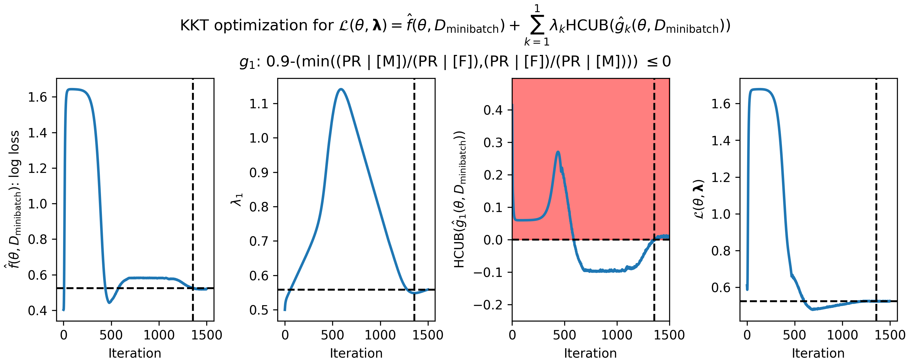 Figure 1 - How the parameters of the KKT optimization problem changed during gradient descent on the loan fairness problem. (Left) primary objective function $\hat{f}(\theta,D_\mathrm{minibatch})$ (in this case the log loss), (middle left) single Lagrange multiplier, ${\lambda_1}$, (middle right) predicted high-confidence upper bound (HCUB) on the disparate impact constraint function, $\hat{g}_1(\theta,D_\mathrm{minibatch})$, and (right) the Lagrangian $\mathcal{L}(\theta,\boldsymbol{\lambda})$. $\boldsymbol{\lambda}$ is in bold here because it is a vector in the general case where there are $n$ constraints. The black dotted lines in each panel indicate where the optimum was found. The optimum is defined as the feasible solution with the lowest value of the primary objective. A feasible solution is one where $\mathrm{HCUB}(\hat{g}_i(\theta,D_\mathrm{cand})) \leq 0, i \in \{1 ... n\}$. In this example, we only have one constraint, and the infeasible region is shown in red in the middle right plot.
Visualizing candidate selection can help you tune the optimization hyperparameters in your spec object. For example, if $\theta$ is never escaping the infeasible region and your Seldonian algorithm is returning NSF (i.e., "No Solution Found"), then you may be able to obtain a solution by running gradient descent (with the Adam optimizer) for more iterations or with different learning rates or velocity values (the beta terms in Adam). If you are still seeing NSF after hyperparameter exploration, you may not have enough data or your constraints may be too strict. Running a Seldonian Experiment can help determine why you are not able to obtain a solution.
Running a Seldonian Experiment
Seldonian Experiments are a way to thoroughly evaluate the performance and safety of Seldonian algorithms, beyond what can be achieved with a single run of the engine. A Seldonian Experiment runs a Seldonian algorithm many times using variable amounts of input data and creates three plots: 1) Performance, 2) Probability of solution, and 3) Probability that the solution violates the constraint as a function of the amount of data used. The Seldonian Experiments library was designed to help implement Seldonian Experiments. We recommend reading the Experiments overview before continuing here. If you have not already installed the Experiments library, follow the instructions here to do so.
To calculate performance and the probability that the solution violates the constraint for any given experimental trial, we need a ground truth dataset. To approximate ground truth, we bootstrap resample from our original dataset and assume that the bootstrap data distribution is the ground truth distribution. While this does not tell you what the performance rate or failure rate will be on your actual problem, it does give a reasonable estimate.
Here is an outline of the experiment we will run:
- Create an array of data fractions, which will determine how much of the data to use as input to the Seldonian algorithm in each trial. We will use 15 different data fractions, which will be log-spaced between 0.001 and 1.0. This array times the number of data points in the original dataset (1000) will make up the horizontal axis of the three plots.
- Create 50 resampled datasets (one for each trial) by sampling with replacement from the dataset we used as input to the engine above. Each resampled dataset will have the same number of rows (1000) as the original dataset. We use 50 trials so that we can compute uncertainties on the plotted quantities at each data fraction. We will use the original dataset as the ground truth dataset for calculating the performance and safety metrics.
-
For each
data_frac in the array of data fractions, run 50 trials. In each trial, use only the first data_frac fraction of the corresponding resampled dataset to run the Seldonian algorithm using the Seldonian Engine. We will use the same spec file we used above for each run of the engine, where only the dataset parameter to SupervisedSpec will be modified for each trial. This will generate 15x50=750 total runs of the Seldonian algorithm. Each run will consist of a different set of fitted model parameters, or "NSF" if no solution was found.
- For each
data_frac, if a solution was returned that passed the safety test, calculate the mean and standard error on the performance (e.g., logistic loss or accuracy) across the 50 trials at this data_frac using the fitted model parameters evaluated on the ground truth dataset. This will be the data used for the first of the three plots. Also record how often a solution was returned and passed the safety test across the 50 trials. This fraction, referred to as the "solution rate", will be used to make the second of the three plots. Finally, for the trials that returned solutions that passed the safety test, calculate the fraction of trials for which the disparate impact statistic, $g_1(\theta)$, was violated, i.e., $g_1(\theta) > 0$, on the ground truth dataset. The fraction violated will be referred to as the "failure rate" and will make up the third and final plot.
We will run this experiment for the Seldonian algorithm as well as for three other models. Two are baseline models: 1) a random classifier that predicts the positive class with probability $p=0.5$ regardless of the input, 2) a simple logistic regression model with no behavioral constraints. The third model comes from another fairness-aware machine learning library called Fairlearn. Fairlearn is not installed by default with the toolkit, for this tutorial we need to install it:
pip install fairlearn==0.7.0
We will describe the Fairlearn model we use in more detail below. Each model requires its own experiment, but the main parameters of the experiment, such as the number of trials and data fractions, as well as the metrics we will calculate (performance, solution rate, and failure rate), are identical. This will allow us to compare the Seldonian algorithm to these other models on the same three plots.
Now, we will show how to implement the described experiment using the Experiments library. At the center of the Experiments library is the PlotGenerator class, and in our particular example, the SupervisedPlotGenerator child class. The goal of the following script is to setup this object, use its methods to run our experiments, and then to make the three plots.
Note: Running the code below in a Jupyter Notebook may crash the notebook. To prevent this from happening, set verbose=False or run the code in a script only.
First, the imports we will need:
import os
os.environ["OMP_NUM_THREADS"] = "1"
import numpy as np
from sklearn.metrics import log_loss

from seldonian.utils.io_utils import load_pickle

from experiments.generate_plots import SupervisedPlotGenerator
from experiments.baselines.logistic_regression import BinaryLogisticRegressionBaseline
from experiments.baselines.random_classifiers import (
    UniformRandomClassifierBaseline)
from experiments.baselines.random_forest import RandomForestClassifierBaseline
Now, we will set up the parameters for the experiments, such as the data fractions we want to use and how many trials at each data fraction we want to run. We will use log-spacing for the data fractions (the horizontal axis of each of the three plots) so that when plotted on a log scale, the data points will be evenly separated. We will use 50 trials at each data fraction so that we can sample a reasonable spread on each quantity at each data fraction.
Fairlearn's fairness definitions are rigid and do not exactly match the definition we used in the engine. To approximate the same definition of disparate impact as ours, we use their definition of demographic parity with a ratio bound of four different values. We will show later that we can change our constraint to match theirs exactly, and the results we find do not change significantly.
Each trial in an experiment is independent of all other trials, so parallelization can speed experiments up enormously. n_workers is how many parallel processes will be used for running the experiments. Set this parameter to however many CPUs you want to use. The line os.environ["OMP_NUM_THREADS"] = "1" in the imports block above turns off NumPy's implicit parallelization, which we want to do when using n_workers>1 (see Tutorial M: Efficient parallelization with the toolkit for more details). Note: using 7 CPUs, this entire script takes 5–10 minutes to run on an M1 Macbook Air. The results for each experiment we run will be saved in subdirectories of results_dir.
if __name__ == "__main__":
    # Parameter setup
    run_experiments = True
    make_plots = True
    save_plot = True
    constraint_name = 'disparate_impact'
    fairlearn_constraint_name = constraint_name
    fairlearn_epsilon_eval = 0.9 # the epsilon used to evaluate g, needs to be same as epsilon in our definition
    fairlearn_eval_method = 'two-groups' # the method for evaluating the Fairlearn model, must match Seldonian constraint definition
    fairlearn_epsilons_constraint = [0.1,1.0,0.9,1.0] # the epsilons used in the fitting constraint
    performance_metric = 'log_loss'
    n_trials = 50
    data_fracs = np.logspace(-3,0,15)
    n_workers = 8
    verbose=True
    results_dir = f'results/loan_{constraint_name}_seldo_log_loss'
    os.makedirs(results_dir,exist_ok=True)

    plot_savename = os.path.join(results_dir,f'{constraint_name}_{performance_metric}.png')
Now, we will need to load the same spec object that we created for running the engine. As before, change the path to the where you saved this file.
   # Load spec
    specfile = f'../engine-repo-dev/examples/loan_tutorial/spec.pkl'
    spec = load_pickle(specfile)
Next, we will set up the ground truth dataset on which we will calculate the performance and the failure rate. In this case, it is just the original dataset.
    # Use entire original dataset as ground truth for test set
    dataset = spec.dataset
    test_features = dataset.features
    test_labels = dataset.labels
We need to define what function perf_eval_fn we will use to evaluate the model's performance. In this case, we will use the logistic (or "log") loss, which happens to be the same as our primary objective. We also define perf_eval_kwargs, which will be passed to the SupervisedPlotGenerator so that we can evaluate the performance evaluation function on the model in each of our experiment trials. Note that this function should be defined outside of the if __name__ == "__main__": block, ideally just above this block. It is shown inside of the block below for illustration purposes only.
    # Setup performance evaluation function and kwargs
    # of the performance evaluation function

    def perf_eval_fn(y_pred,y,**kwargs):
        return log_loss(y,y_pred)

    perf_eval_kwargs = {
        'X':test_features,
        'y':test_labels,
        }
Now we instantiate the plot generator, passing in the parameters from variables we defined above.
    plot_generator = SupervisedPlotGenerator(
        spec=spec,
        n_trials=n_trials,
        data_fracs=data_fracs,
        n_workers=n_workers,
        datagen_method='resample',
        perf_eval_fn=perf_eval_fn,
        constraint_eval_fns=[],
        results_dir=results_dir,
        perf_eval_kwargs=perf_eval_kwargs,
        )
We will first run our two baseline experiments, which we can do by calling the run_baseline_experiment() method of the plot generator and passing in the baseline model name of choice.
    # Baseline models
    if run_experiments:
        plot_generator.run_baseline_experiment(
            baseline_model=UniformRandomClassifierBaseline(),verbose=verbose)

        plot_generator.run_baseline_experiment(
            baseline_model=BinaryLogisticRegressionBaseline(),verbose=verbose)
Similarly, to run our Seldonian Experiment, we call the corresponding method of the plot generator:
        # Seldonian experiment
        plot_generator.run_seldonian_experiment(verbose=verbose)
The last experiment we will run is the Fairlearn experiment. While Fairlearn does not explictly support a a disparate impact constraint, disparate impact can be constructed using their demographic parity constraint with a ratio bound. Under the hood, we are using the following Fairlearn model, where fairlearn_epsilon_constraint is one of the four values in the list we defined above. Note that the following code is not part of the experiment script and you do not need to run it. It is shown only to illuminate how we are implementing the Fairlearn model in our experiment.
from sklearn.linear_model import LogisticRegression
from fairlearn.reductions import ExponentiatedGradient
from fairlearn.reductions import DemographicParity
fairlearn_constraint = DemographicParity(
                ratio_bound=fairlearn_epsilon_constraint)
classifier = LogisticRegression()
mitigator = ExponentiatedGradient(classifier,
            fairlearn_constraint)
The way Fairlearn handles sensitive columns is different than way we handle them in the Seldonian Engine library. In the engine, we one-hot encode sensitive columns. In Fairlearn, they integer encode. This is why we have two columns, M and F, in the dataset used for the engine, whereas they would have one for defining the sex. It turns out that our M column encodes both sexes since it is binary-valued (0=female, 1=male), so we can just tell Fairlearn to use the "M" column. Our script continues with the following code.
    ######################
    # Fairlearn experiment
    ######################

    fairlearn_sensitive_feature_names = ['M']
    fairlearn_sensitive_col_indices = [dataset.sensitive_col_names.index(
        col) for col in fairlearn_sensitive_feature_names]
    fairlearn_sensitive_features = dataset.sensitive_attrs[:,fairlearn_sensitive_col_indices]
    # Setup ground truth test dataset for Fairlearn
    test_features_fairlearn = test_features
    fairlearn_eval_kwargs = {
        'X':test_features_fairlearn,
        'y':test_labels,
        'sensitive_features':fairlearn_sensitive_features,
        'eval_method':fairlearn_eval_method,
        }

    if run_experiments:
        for fairlearn_epsilon_constraint in fairlearn_epsilons_constraint:
            plot_generator.run_fairlearn_experiment(
                verbose=verbose,
                fairlearn_sensitive_feature_names=fairlearn_sensitive_feature_names,
                fairlearn_constraint_name=fairlearn_constraint_name,
                fairlearn_epsilon_constraint=fairlearn_epsilon_constraint,
                fairlearn_epsilon_eval=fairlearn_epsilon_eval,
                fairlearn_eval_kwargs=fairlearn_eval_kwargs,
                )
Now that the experiments have been run, we can make the three plots. At the top of the script, we set save_plot = False, so while the plot will be displayed to the screen, it will not be saved. Setting save_plot = True at the top of the script will save the plot to disk but will not display it to screen.
    if make_plots:
        plot_generator.make_plots(fontsize=12,legend_fontsize=10,
            performance_label=performance_metric,
            performance_yscale='log',
            model_label_dict=model_label_dict,
            savename=plot_savename if save_plot else None,
            save_format="png")
Here is the entire script all together, which we will call generate_threeplots.py:
Note: Running the code below in a Jupyter Notebook may crash the notebook. To prevent this from happening, set verbose=False or run the code in a script only.
import os
import numpy as np

from experiments.generate_plots import SupervisedPlotGenerator
from seldonian.utils.io_utils import load_pickle
from sklearn.metrics import log_loss

def perf_eval_fn(y_pred,y,**kwargs):
    return log_loss(y,y_pred)

if __name__ == "__main__":
    # Parameter setup
    run_experiments = True
    make_plots = True
    save_plot = True
    constraint_name = 'disparate_impact'
    fairlearn_constraint_name = constraint_name
    fairlearn_epsilon_eval = 0.9 # the epsilon used to evaluate g, needs to be same as epsilon in our definition
    fairlearn_eval_method = 'two-groups' # the epsilon used to evaluate g, needs to be same as epsilon in our definition
    fairlearn_epsilons_constraint = [0.01,0.1,0.9,1.0] # the epsilons used in the fitting constraint
    performance_metric = 'log_loss'
    n_trials = 50
    data_fracs = np.logspace(-3,0,15)
    n_workers = 8
    verbose=True
    results_dir = f'results/loan_{constraint_name}_seldodef_log_loss_debug_2022Nov6'
    os.makedirs(results_dir,exist_ok=True)

    plot_savename = os.path.join(results_dir,f'{constraint_name}_{performance_metric}.png')

    # Load spec
    specfile = f'../engine-repo-dev/examples/loan_tutorial/spec.pkl'
    spec = load_pickle(specfile)

    # Use entire original dataset as ground truth for test set
    dataset = spec.dataset
    test_features = dataset.features
    test_labels = dataset.labels

    # Setup performance evaluation function and kwargs
    # of the performance evaluation function

    perf_eval_kwargs = {
        'X':test_features,
        'y':test_labels,
        }

    plot_generator = SupervisedPlotGenerator(
        spec=spec,
        n_trials=n_trials,
        data_fracs=data_fracs,
        n_workers=n_workers,
        datagen_method='resample',
        perf_eval_fn=perf_eval_fn,
        constraint_eval_fns=[],
        results_dir=results_dir,
        perf_eval_kwargs=perf_eval_kwargs,
        )

    if run_experiments:
        # Baseline models
        plot_generator.run_baseline_experiment(
            baseline_model=UniformRandomClassifierBaseline,verbose=verbose)

        plot_generator.run_baseline_experiment(
            baseline_model=BinaryLogisticRegressionBaseline,verbose=verbose)

        # Seldonian experiment
        plot_generator.run_seldonian_experiment(verbose=verbose)

    ######################
    # Fairlearn experiment
    ######################
    fairlearn_sensitive_feature_names = ['M']
    fairlearn_sensitive_col_indices = [dataset.sensitive_col_names.index(
        col) for col in fairlearn_sensitive_feature_names]
    fairlearn_sensitive_features = dataset.sensitive_attrs[:,fairlearn_sensitive_col_indices]
    # Setup ground truth test dataset for Fairlearn
    test_features_fairlearn = test_features
    fairlearn_eval_kwargs = {
        'X':test_features_fairlearn,
        'y':test_labels,
        'sensitive_features':fairlearn_sensitive_features,
        'eval_method':fairlearn_eval_method,
        }

    if run_experiments:
        for fairlearn_epsilon_constraint in fairlearn_epsilons_constraint:
            plot_generator.run_fairlearn_experiment(
                verbose=verbose,
                fairlearn_sensitive_feature_names=fairlearn_sensitive_feature_names,
                fairlearn_constraint_name=fairlearn_constraint_name,
                fairlearn_epsilon_constraint=fairlearn_epsilon_constraint,
                fairlearn_epsilon_eval=fairlearn_epsilon_eval,
                fairlearn_eval_kwargs=fairlearn_eval_kwargs,
                )

    if make_plots:
        plot_generator.make_plots(fontsize=12,legend_fontsize=10,
            performance_label=performance_metric,
            performance_yscale='log',
            model_label_dict=model_label_dict,
            savename=plot_savename if save_plot else None,
            save_format="png")
Running the script will produce the following plot (or something very similar depending on your machine's random number generator):
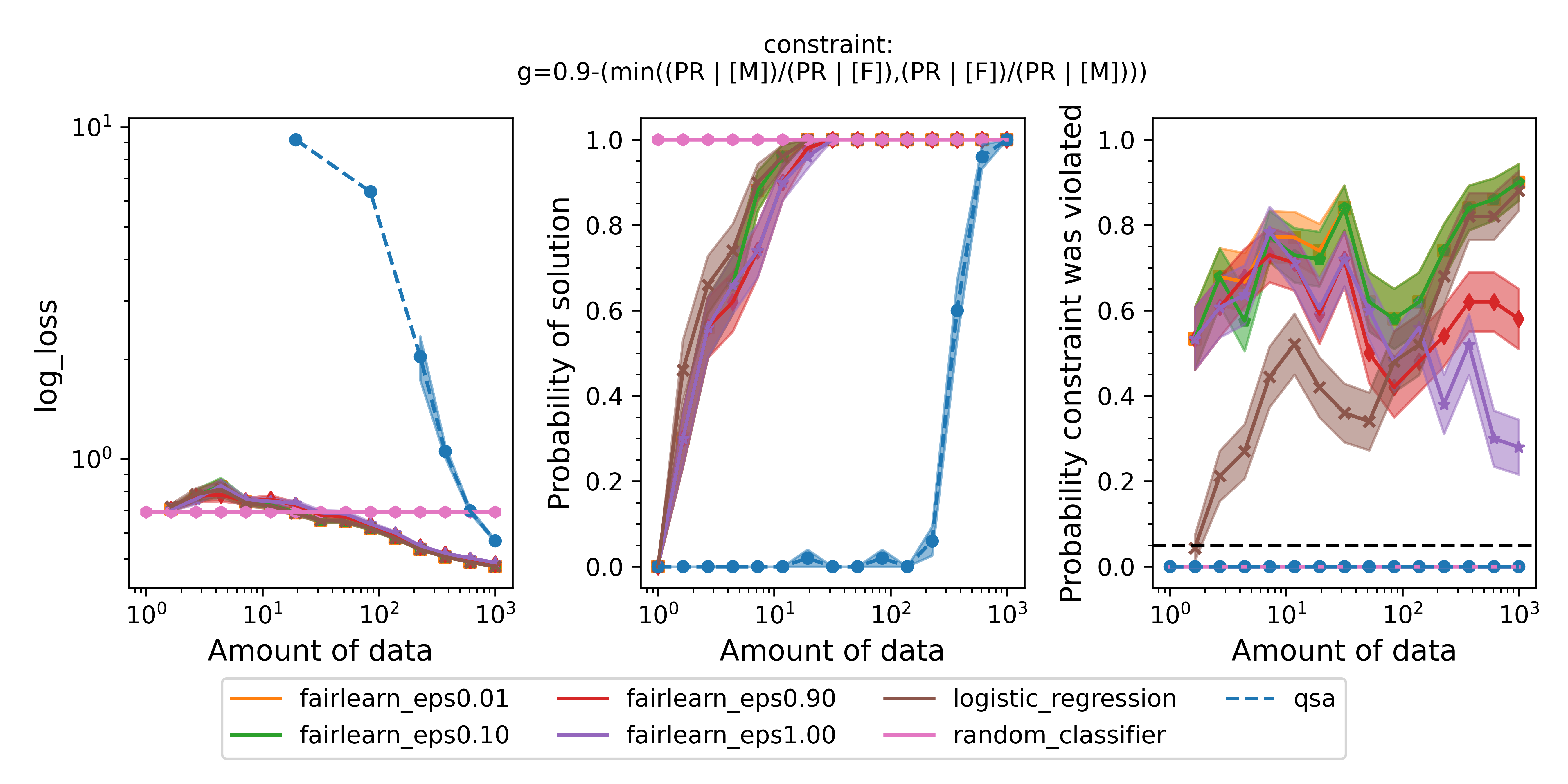 Figure 2 - The three plots of a Seldonian Experiment shown for the UCI German Credit dataset. The disparate impact fairness constraint, $g$, is written at the top of the figure. When $g\leq0$, the fairness constraint is satisfied. Each panel shows the mean (point) and standard error (shaded region) of a quantity as a function of the size of the training set (determined from the data fraction array) for several models: the quasi-Seldonian model (QSA, blue), the two baseline models: 1) a random classifier (pink) that predicts the positive class with $p=0.5$ every time and 2) a logistic regression model without any constraints added (brown), and a Fairlearn model with four different values of epsilon, the ratio bound. (Left) the logistic loss. (Middle) the fraction of trials that returned a solution. (Right) the fraction of trials that violated the safety constraint on the ground truth dataset. The black dashed line is set at the $\delta=0.05$ value that we set in our behavioral constraint.
The QSA takes more data to return a solution (middle panel) than the other models because it makes a high-confidence guarantee that the solution it returns will be safe. That guarantee is validated because the QSA never violates the fairness constraint on the ground truth dataset (right panel). The QSA's performance (left panel) approaches the performance of the logistic regression baseline as the number of training samples approaches 1000, the size of the original dataset. The logistic regression model and even the fairness-aware Fairlearn model return solutions with less data, but both violate the constraint quite often. This is true for all four values of the disparate impact threshold, epsilon, and despite the fact that Fairlearn is using a behavioral constraint analogous to disparate impact. The fact that the QSA never returns a solution with probability of 1.0 underscores that Seldonian algorithms often need a reasonable amount of data ($\gt1000$) to return solutions. The precise amount of data needed will depend on the dataset and constraint(s), and determining that amount is one of the reasons to run a Seldonian Experiment.
Some minor points of these plots are:
- The performance is not plotted for trials that did not return a solution. For the smallest data fractions (e.g., 0.001), only the random classifier returns a solution because it is defined to always return the same solution independent of input.
- The solution rate is between 0 and 1 for the logistic regression model and the Fairlearn models for small amounts of data, not 0 or 1 as one might expect. This happens because in each trial, at a fixed number of training samples, a different resampled dataset is used. When the number of training samples is small ($\lesssim 10$), some of these resampled datasets only contain data labeled for one of the two label classes, i.e., all 0s or all 1s. The logistic regression model and the Fairlearn models return an error when we attempt to train them on these datasets. We count those cases as not returning a solution. Note that Seldonian algorithms do not return a solution for a different reason. They do this when the algorithm deems that the solution is not safe. The random classifier does not use the input data to make predictions, which is why it always returns a solution.
- The failure rate is not plotted for trials that did not return a solution for all models except QSA. The logistic regression baseline and Fairlearn can fail to converge, for example. However, the QSA will always return either a solution or "NSF", even when only one data point (i.e.,
data_frac=0.001) is provided as input. In cases where it returns "NSF", that solution is considered safe.
- The random classifier does not violate the safety constraint ever because its positive rate is 0.5 for all datapoints, regardless of sex.
Modifying the constraint to line up with Fairlearn's constraint
We mentioned that Fairlearn cannot exactly enforce the disparate impact constraint we defined: $\text{min}( (\text{PR} | [\text{M}]) / (\text{PR} | [\text{F}]), (\text{PR} | [\text{F}]) / (\text{PR} | [\text{M}]) ) \geq 0.9$. This is because Fairlearn's fairness constraints for binary classification only compare statistics like positive rate between a single group (such as "male") in a protected class (such as gender) and the mean of all groups in that class. The Seldonian Engine is flexible in how its constraints can be defined, and we can tweak our disparate impact constraint definition to match the Fairlearn definition. To match the Fairlearn definition, our constraint must take the form: $\text{min}( (\text{PR} | [\text{M}]) / (\text{PR}), (\text{PR}) / (\text{PR} | [\text{M}]) ) \geq 0.9$, where the only thing we have changed from our original constraint is substituting $(\text{PR} | [\text{F}])$ (positive rate, given female) in our original constraint for $(\text{PR})$, the mean positive rate.
Let us rerun the same experiment above with this new constraint. First, we need to create a new spec file, where the only difference is the constraint definition. This will build a new parse tree from the new constraint. Replace the line in createSpec.py above:
# Define behavioral constraints
constraint_strs = ['min((PR | [M])/(PR | [F]),(PR | [F])/(PR | [M])) >= 0.9']
with:
# Define behavioral constraints
constraint_strs = ['min((PR | [M])/(PR),(PR)/(PR | [M])) >= 0.9']
Then, change the line where the spec file is saved so it does not overwrite the old spec file from:
spec_save_name = os.path.join(save_dir,'spec.pkl')
to something like:
spec_save_name = os.path.join(save_dir,'spec_fairlearndef.pkl')
Once that file is saved, you are ready to run the experiments again. There are only a few changes you will need to make to the file generate_threeplots.py. They are:
- Set
fairlearn_eval_method = "native".
- Set
fairlearn_epsilons_constraint = [0.9].
- Point
specfile to the new spec file you just created.
- Change
results_dir to a new directory so you do not overwrite the results from the previous experiment.
Running the script with these changes will produce a plot that should look very similar to this:
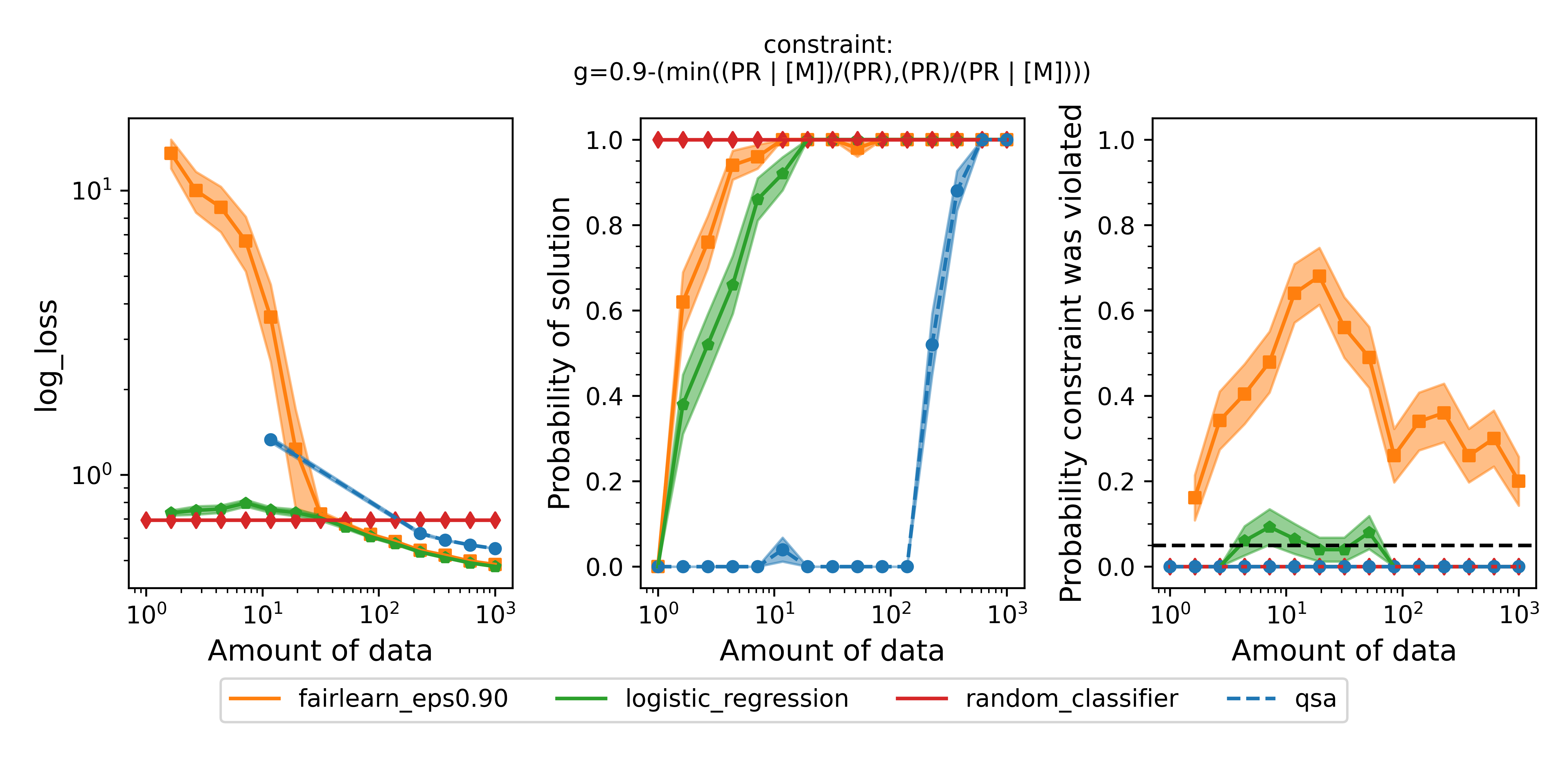 Figure 3 - Same as Figure 2 but with the definition of disparate impact that Fairlearn uses, i.e., $\text{min}( (\text{PR} | [\text{M}]) / (\text{PR}), (\text{PR}) / (\text{PR} | [\text{M}]) ) \geq 0.9$. In this experiment, we used a single Fairlearn model with $\epsilon=0.9$ because the constraint was identical to the constraint used in the QSA model, which was not true in the previous set of experiments.
The results are very similar to the previous experiments. As before, the QSA takes more data than the baselines and Fairlearn to return solutions, but those solutions are safe. The solutions from the Fairlearn model are frequently unsafe.
We could use the same procedure we just carried out to change the fairness definition entirely. For example, another common definition of fairness is equalized odds, which ensures that the false positive rates and false negative rates simultaneously do not differ within a certain tolerance. Let's define the constraint string that the engine can understand: $\text{abs}((\text{FPR} | [\text{M}]) - (\text{FPR} | [\text{F}])) + \text{abs}((\text{FNR} | [\text{M}]) - (\text{FNR} | [\text{F}])) \leq 0.2$. Repeating the same procedure as above to replace the constraint with this one and create a new spec file, the only changes we need to make to the experiment script are:
constraint_name = 'equalized_odds'
fairlearn_constraint_name = constraint_name
fairlearn_epsilon_eval = 0.2 # the epsilon used to evaluate g, needs to be same as epsilon in our definition
fairlearn_eval_method = 'two-groups' # the epsilon used to evaluate g, needs to be same as epsilon in our definition
fairlearn_epsilons_constraint = [0.01,0.1,0.2,1.0] # the epsilons used in the fitting constraint
We also need to point to the new spec file we created for the new constraint. Running the experiment for this constraint, we obtain the following figure:
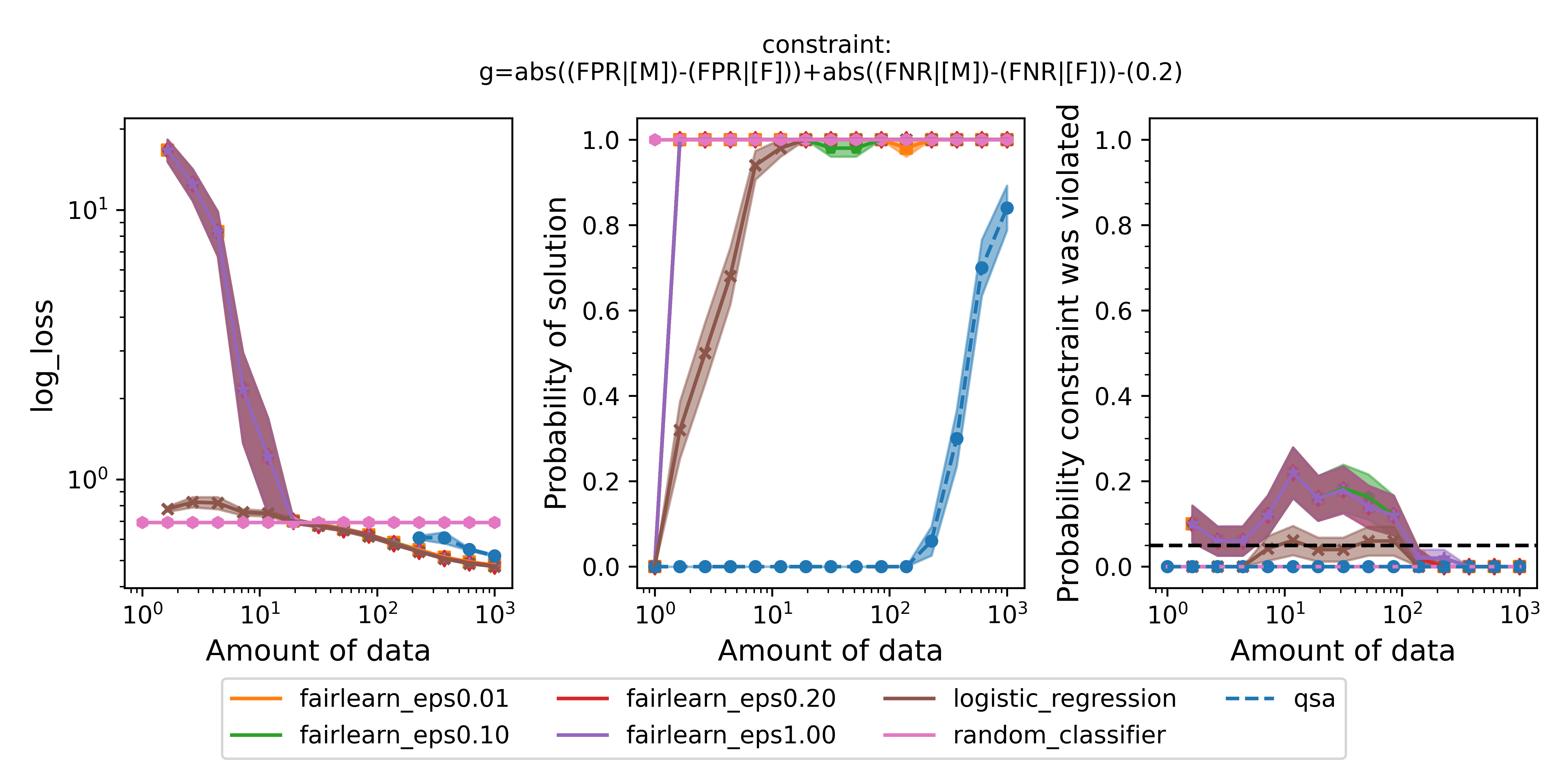 Figure 4 - Same as Figure 2 but enforcing equalized odds instead of disparate impact.
Summary
In this tutorial, we demonstrated how to use the Seldonian Toolkit to build a predictive model that enforces a variety of fairness constraints on the German Credit dataset. We covered how to format the dataset and metadata so that they can be used by the Seldonian Engine. Using the engine, we ran a Seldonian algorithm and confirmed that we were able to find a safe solution. We then ran a serires of Seldonian Experiments to evaluate the true performance and safety of our quasi-Seldonian algorithm (QSA) using different fairness definitions.
We found that the QSA can flexibly satisfy a range of custom-defined fairness constraints and that the model does not violate the constraints. We compared the QSA to several baselines that do not enforce any behavioral constraints as well as one model, Fairlearn, that does enforce constraints. We found that the performance of the QSA approaches the performance of a logistic regression model that lacks constraints. The logistic regression model and the fairness-aware Fairlearn model frequently violate the constraints for some definitions of fairness.